DeepExtractor — Training Tutorial (Google Colab)¶

This notebook trains a fresh DeepExtractor model from scratch on synthetic (numpy) noise, plots the training losses, and tests the model on sine-Gaussian injections. It is designed to run on Google Colab with a free T4 GPU.

Tip: Go to Runtime → Change runtime type → GPU before running.

[ ]:

!pip install deepextractor

[7]:

import os
import numpy as np
import torch
import torch.nn as nn
import torch.optim as optim
import matplotlib.pyplot as plt
from sklearn.preprocessing import StandardScaler
from torch.optim.lr_scheduler import ReduceLROnPlateau

import warnings
warnings.filterwarnings("ignore", "Wswiglal-redir-stdio")

from deepextractor.models.architectures import UNET2D
from deepextractor.generation.generate_timeseries import (
    generate_gaussian_noise, generate_synthetic_data, LENGTH, SAMPLE_RATE, T
)
from deepextractor.generation.glitch_functions import generate_sine_gaussian
from deepextractor.utils.signal import whitened_snr_scaling
from deepextractor.training.train_fn import train_fn
from deepextractor.utils.io import check_accuracy

Configuration¶

[38]:

# Device — uses MPS on Apple Silicon, CUDA on Linux/Windows GPU, otherwise CPU
if torch.cuda.is_available():
    DEVICE = "cuda"
elif torch.backends.mps.is_available():
    DEVICE = "mps"
else:
    DEVICE = "cpu"
print(f"Using device: {DEVICE}")

# Dataset size — keep small for a quick demo; increase for real training
N_TRAIN = 1000
N_VAL   = 200

# Training
BATCH_SIZE              = 32
EPOCHS                  = 50    # maximum epochs; early stopping may stop sooner however, this specific architecture will likely converge at a much higher epoch
LR                      = 1e-4
LR_PATIENCE             = 4     # epochs without improvement before LR is reduced
LR_FACTOR               = 0.1   # factor to reduce LR by
EARLY_STOPPING_PATIENCE = 9     # epochs without improvement before training stops

# STFT parameters
# Original DeepExtractor (arXiv:2501.18423): N_FFT=512, WIN_LENGTH=64, HOP_LENGTH=32
# → produces (257, 257) spectrograms, richer time-frequency representation
#   but significantly slower to train.
# Tutorial default: smaller spectrograms for faster training, but still gives decent performance (please see 129x129 model in the paper).
N_FFT      = 256
WIN_LENGTH = N_FFT // 2
HOP_LENGTH = WIN_LENGTH // 2

# Physical time axis — Mojito/LISA-compatible (0.5 Hz, dt = 2.0 s per sample)
DT         = 1.0 / 0.5          # seconds per sample  =  2.0 s
T_PHYSICAL = LENGTH * DT        # total window duration = 16384 s

Using device: mps

Step 1 — Generate synthetic time-domain data¶

Each training sample is a pair:

Input glitch: background noise with 1–30 synthetic signal injections (chirps, sine-Gaussians, etc.)
Target background: the same noise without any injections

The model learns to map glitchy strain → clean background.

[9]:

mean, std_dev = 0, np.sqrt(SAMPLE_RATE / 2)  # PyCBC convention: variance = SAMPLE_RATE / 2

print("Generating training noise...")
train_noise = generate_gaussian_noise(mean, std_dev, N_TRAIN, (LENGTH,), bilby_noise=False)
print("Generating validation noise...")
val_noise   = generate_gaussian_noise(mean, std_dev, N_VAL,   (LENGTH,), bilby_noise=False)

print("Generating training pairs...")
glitch_train, bg_train = generate_synthetic_data(train_noise, bilby_noise=False, phase="train")
print("Generating validation pairs...")
glitch_val,   bg_val   = generate_synthetic_data(val_noise,   bilby_noise=False, phase="val")

print(f"\nTrain: {glitch_train.shape}  |  Val: {glitch_val.shape}")

Generating training noise...
Generating pycbc noise...
Generating validation noise...
Generating pycbc noise...
Generating training pairs...

Generating Synthetic Train Data: 100%|██████████| 1000/1000 [00:03<00:00, 306.30it/s]

Generating validation pairs...

Generating Synthetic Val Data: 100%|██████████| 200/200 [00:00<00:00, 269.64it/s]


Train: (1000, 8192)  |  Val: (200, 8192)

Step 2 — Scale and convert to spectrograms¶

[10]:

scaler = StandardScaler()
glitch_train_scaled = scaler.fit_transform(glitch_train.reshape(-1, 1)).reshape(glitch_train.shape)
bg_train_scaled     = scaler.transform(bg_train.reshape(-1, 1)).reshape(bg_train.shape)
glitch_val_scaled   = scaler.transform(glitch_val.reshape(-1, 1)).reshape(glitch_val.shape)
bg_val_scaled       = scaler.transform(bg_val.reshape(-1, 1)).reshape(bg_val.shape)

# Uncomment to save the scaler for use outside this notebook
# import pickle, os
# os.makedirs('/tmp/de_training_tutorial', exist_ok=True)
# with open('/tmp/de_training_tutorial/scaler.pkl', 'wb') as f:
#     pickle.dump(scaler, f)

# Convert to STFT spectrograms (in-memory)
window = torch.hann_window(WIN_LENGTH)

def to_mag_phase(arrays):
    """Convert a numpy array (N, time) to a (N, 2, F, T) mag/phase tensor."""
    t = torch.tensor(arrays, dtype=torch.float32)
    stft = torch.stft(t, n_fft=N_FFT, hop_length=HOP_LENGTH, win_length=WIN_LENGTH,
                      window=window, return_complex=True)
    mag   = torch.abs(stft)
    phase = torch.angle(stft)
    return torch.stack([mag, phase], dim=1)  # (N, 2, F, T)

glitch_train_spec = to_mag_phase(glitch_train_scaled)
bg_train_spec     = to_mag_phase(bg_train_scaled)
glitch_val_spec   = to_mag_phase(glitch_val_scaled)
bg_val_spec       = to_mag_phase(bg_val_scaled)

print(f"Spectrogram shape: {glitch_train_spec.shape}  — (N, 2, freq_bins, time_bins)")

# Uncomment to save spectrograms to disk (useful for large datasets or re-use)
# os.makedirs('/tmp/de_training_tutorial/spectrogram_domain', exist_ok=True)
# for name, arr in [
#     ('glitch_train_scaled_mag_phase',     glitch_train_spec.numpy()),
#     ('background_train_scaled_mag_phase', bg_train_spec.numpy()),
#     ('glitch_val_scaled_mag_phase',       glitch_val_spec.numpy()),
#     ('background_val_scaled_mag_phase',   bg_val_spec.numpy()),
# ]:
#     np.save(f'/tmp/de_training_tutorial/spectrogram_domain/{name}', arr)

Spectrogram shape: torch.Size([1000, 2, 129, 129])  — (N, 2, freq_bins, time_bins)

Step 3 — Build model and data loaders¶

[11]:

from torch.utils.data import TensorDataset, DataLoader

# Model architecture
# Original DeepExtractor (arXiv:2501.18423): features=[64, 128, 256, 512] — ~31M parameters.
# Use those to train a model equivalent to the published DeepExtractor.
# Tutorial default: one fewer layer and half the filters for faster training.
model = UNET2D(in_channels=2, out_channels=2, features=[32, 64, 128, 256]).to(DEVICE)
print(f"Model parameters: {sum(p.numel() for p in model.parameters()):,}")

train_ds = TensorDataset(glitch_train_spec, bg_train_spec)
val_ds   = TensorDataset(glitch_val_spec,   bg_val_spec)

train_loader = DataLoader(train_ds, batch_size=BATCH_SIZE, shuffle=True)
val_loader   = DataLoader(val_ds,   batch_size=BATCH_SIZE, shuffle=False)

print(f"Train batches: {len(train_loader)}  |  Val batches: {len(val_loader)}")
print(f"Spectrogram shape: {glitch_train_spec.shape}  — (N, 2, freq_bins, time_bins)")

Model parameters: 7,762,786
Train batches: 32  |  Val batches: 7
Spectrogram shape: torch.Size([1000, 2, 129, 129])  — (N, 2, freq_bins, time_bins)

Step 4 — Train¶

We train the network for up to EPOCHS iterations. For this minimal tutorial configuration (1000 samples, reduced model), 50 epochs is sufficient to see the loss converge. To train a model to full convergence, set EPOCHS to a large number (e.g. 200) — the learning rate scheduler and early stopping will halt training automatically once the validation loss stops improving. For longer runs, we recommend using a CUDA GPU (e.g. Google Colab).

[12]:

loss_fn   = nn.MSELoss()
optimizer = optim.Adam(model.parameters(), lr=LR)
scheduler = ReduceLROnPlateau(optimizer, mode="min", factor=LR_FACTOR, patience=LR_PATIENCE)
amp_scaler = torch.amp.GradScaler("cuda") if DEVICE == "cuda" else torch.amp.GradScaler("cpu", enabled=False)

train_losses, val_losses = [], []
best_val_loss           = float("inf")
early_stopping_counter  = 0

for epoch in range(EPOCHS):
    train_loss, _, _ = train_fn(
        train_loader, model, "DeepExtractor_257", optimizer, loss_fn, amp_scaler, DEVICE
    )
    val_loss, _, _ = check_accuracy(val_loader, model, "DeepExtractor_257", device=DEVICE)

    train_losses.append(train_loss)
    val_losses.append(val_loss)
    scheduler.step(val_loss)

    current_lr = optimizer.param_groups[0]['lr']
    print(f"Epoch {epoch+1:>3}/{EPOCHS}  train={train_loss:.5f}  val={val_loss:.5f}  lr={current_lr:.1e}")

    if val_loss < best_val_loss:
        best_val_loss          = val_loss
        early_stopping_counter = 0
    else:
        early_stopping_counter += 1
        if early_stopping_counter >= EARLY_STOPPING_PATIENCE:
            print(f"\nEarly stopping at epoch {epoch+1} (no improvement for {EARLY_STOPPING_PATIENCE} epochs).")
            break

print("\nTraining complete.")

Training on batch: 100%|██████████| 32/32 [00:12<00:00,  2.65it/s, loss=1.44]

Validation Loss: 1.642826
Epoch   1/50  train=1.78164  val=1.64283  lr=1.0e-04

Training on batch: 100%|██████████| 32/32 [00:09<00:00,  3.20it/s, loss=1.06]

Validation Loss: 1.046674
Epoch   2/50  train=1.20411  val=1.04667  lr=1.0e-04

Training on batch: 100%|██████████| 32/32 [00:10<00:00,  3.15it/s, loss=0.99]

Validation Loss: 0.898930
Epoch   3/50  train=0.97752  val=0.89893  lr=1.0e-04

Training on batch: 100%|██████████| 32/32 [00:10<00:00,  3.17it/s, loss=0.899]

Validation Loss: 0.817464
Epoch   4/50  train=0.86443  val=0.81746  lr=1.0e-04

Training on batch: 100%|██████████| 32/32 [00:10<00:00,  3.15it/s, loss=0.823]

Validation Loss: 0.756312
Epoch   5/50  train=0.79319  val=0.75631  lr=1.0e-04

Training on batch: 100%|██████████| 32/32 [00:10<00:00,  3.15it/s, loss=0.626]

Validation Loss: 0.719852
Epoch   6/50  train=0.73717  val=0.71985  lr=1.0e-04

Training on batch: 100%|██████████| 32/32 [00:10<00:00,  3.15it/s, loss=0.731]

Validation Loss: 0.676591
Epoch   7/50  train=0.70375  val=0.67659  lr=1.0e-04

Training on batch: 100%|██████████| 32/32 [00:10<00:00,  3.15it/s, loss=0.747]

Validation Loss: 0.651633
Epoch   8/50  train=0.68063  val=0.65163  lr=1.0e-04

Training on batch: 100%|██████████| 32/32 [00:10<00:00,  3.02it/s, loss=0.627]

Validation Loss: 0.630227
Epoch   9/50  train=0.65432  val=0.63023  lr=1.0e-04

Training on batch: 100%|██████████| 32/32 [00:10<00:00,  3.15it/s, loss=0.784]

Validation Loss: 0.611459
Epoch  10/50  train=0.64097  val=0.61146  lr=1.0e-04

Training on batch: 100%|██████████| 32/32 [00:10<00:00,  3.15it/s, loss=0.795]

Validation Loss: 0.600421
Epoch  11/50  train=0.62777  val=0.60042  lr=1.0e-04

Training on batch: 100%|██████████| 32/32 [00:10<00:00,  3.01it/s, loss=0.658]

Validation Loss: 0.592885
Epoch  12/50  train=0.61680  val=0.59288  lr=1.0e-04

Training on batch: 100%|██████████| 32/32 [00:10<00:00,  2.95it/s, loss=0.526]

Validation Loss: 0.582830
Epoch  13/50  train=0.60304  val=0.58283  lr=1.0e-04

Training on batch: 100%|██████████| 32/32 [00:10<00:00,  3.01it/s, loss=0.753]

Validation Loss: 0.574770
Epoch  14/50  train=0.59984  val=0.57477  lr=1.0e-04

Training on batch: 100%|██████████| 32/32 [00:10<00:00,  3.02it/s, loss=0.604]

Validation Loss: 0.570096
Epoch  15/50  train=0.58922  val=0.57010  lr=1.0e-04

Training on batch: 100%|██████████| 32/32 [00:10<00:00,  3.03it/s, loss=0.7]

Validation Loss: 0.566964
Epoch  16/50  train=0.58518  val=0.56696  lr=1.0e-04

Training on batch: 100%|██████████| 32/32 [00:10<00:00,  3.00it/s, loss=0.726]

Validation Loss: 0.561656
Epoch  17/50  train=0.58561  val=0.56166  lr=1.0e-04

Training on batch: 100%|██████████| 32/32 [00:10<00:00,  2.95it/s, loss=0.53]

Validation Loss: 0.558215
Epoch  18/50  train=0.57418  val=0.55821  lr=1.0e-04

Training on batch: 100%|██████████| 32/32 [00:11<00:00,  2.89it/s, loss=0.498]

Validation Loss: 0.554613
Epoch  19/50  train=0.56821  val=0.55461  lr=1.0e-04

Training on batch: 100%|██████████| 32/32 [00:11<00:00,  2.84it/s, loss=0.661]

Validation Loss: 0.551478
Epoch  20/50  train=0.56811  val=0.55148  lr=1.0e-04

Training on batch: 100%|██████████| 32/32 [00:12<00:00,  2.57it/s, loss=0.626]

Validation Loss: 0.548884
Epoch  21/50  train=0.56340  val=0.54888  lr=1.0e-04

Training on batch: 100%|██████████| 32/32 [00:11<00:00,  2.73it/s, loss=0.613]

Validation Loss: 0.547886
Epoch  22/50  train=0.55910  val=0.54789  lr=1.0e-04

Training on batch: 100%|██████████| 32/32 [00:11<00:00,  2.72it/s, loss=0.714]

Validation Loss: 0.545268
Epoch  23/50  train=0.55753  val=0.54527  lr=1.0e-04

Training on batch: 100%|██████████| 32/32 [00:11<00:00,  2.69it/s, loss=0.528]

Validation Loss: 0.544565
Epoch  24/50  train=0.54982  val=0.54457  lr=1.0e-04

Training on batch: 100%|██████████| 32/32 [00:11<00:00,  2.67it/s, loss=0.555]

Validation Loss: 0.543454
Epoch  25/50  train=0.54636  val=0.54345  lr=1.0e-04

Training on batch: 100%|██████████| 32/32 [00:12<00:00,  2.65it/s, loss=0.591]

Validation Loss: 0.542992
Epoch  26/50  train=0.54280  val=0.54299  lr=1.0e-04

Training on batch: 100%|██████████| 32/32 [00:12<00:00,  2.65it/s, loss=0.503]

Validation Loss: 0.542006
Epoch  27/50  train=0.53653  val=0.54201  lr=1.0e-04

Training on batch: 100%|██████████| 32/32 [00:13<00:00,  2.40it/s, loss=0.626]

Validation Loss: 0.541491
Epoch  28/50  train=0.53514  val=0.54149  lr=1.0e-04

Training on batch: 100%|██████████| 32/32 [00:12<00:00,  2.49it/s, loss=0.596]

Validation Loss: 0.542764
Epoch  29/50  train=0.53112  val=0.54276  lr=1.0e-04

Training on batch: 100%|██████████| 32/32 [00:12<00:00,  2.48it/s, loss=0.506]

Validation Loss: 0.540388
Epoch  30/50  train=0.52469  val=0.54039  lr=1.0e-04

Training on batch: 100%|██████████| 32/32 [00:13<00:00,  2.45it/s, loss=0.64]

Validation Loss: 0.541270
Epoch  31/50  train=0.52259  val=0.54127  lr=1.0e-04

Training on batch: 100%|██████████| 32/32 [00:12<00:00,  2.48it/s, loss=0.544]

Validation Loss: 0.541796
Epoch  32/50  train=0.51645  val=0.54180  lr=1.0e-04

Training on batch: 100%|██████████| 32/32 [00:12<00:00,  2.57it/s, loss=0.469]

Validation Loss: 0.542653
Epoch  33/50  train=0.51006  val=0.54265  lr=1.0e-04

Training on batch: 100%|██████████| 32/32 [00:12<00:00,  2.56it/s, loss=0.395]

Validation Loss: 0.542553
Epoch  34/50  train=0.50551  val=0.54255  lr=1.0e-04

Training on batch: 100%|██████████| 32/32 [00:12<00:00,  2.59it/s, loss=0.499]

Validation Loss: 0.543155
Epoch  35/50  train=0.50300  val=0.54315  lr=1.0e-05

Training on batch: 100%|██████████| 32/32 [00:12<00:00,  2.60it/s, loss=0.51]

Validation Loss: 0.541909
Epoch  36/50  train=0.49521  val=0.54191  lr=1.0e-05

Training on batch: 100%|██████████| 32/32 [00:12<00:00,  2.60it/s, loss=0.46]

Validation Loss: 0.542595
Epoch  37/50  train=0.49076  val=0.54259  lr=1.0e-05

Training on batch: 100%|██████████| 32/32 [00:12<00:00,  2.58it/s, loss=0.422]

Validation Loss: 0.543145
Epoch  38/50  train=0.48851  val=0.54315  lr=1.0e-05

Training on batch: 100%|██████████| 32/32 [00:12<00:00,  2.57it/s, loss=0.67]

Validation Loss: 0.543338
Epoch  39/50  train=0.49375  val=0.54334  lr=1.0e-05

Early stopping at epoch 39 (no improvement for 9 epochs).

Training complete.

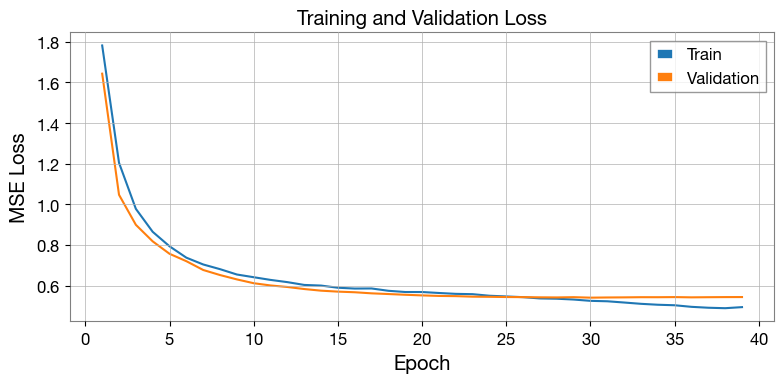
Step 5 — Plot losses¶

[13]:

epochs_ran = range(1, len(train_losses) + 1)

fig, ax = plt.subplots(figsize=(8, 4))
ax.plot(epochs_ran, train_losses, label="Train",      color="C0")
ax.plot(epochs_ran, val_losses,   label="Validation", color="C1")
ax.set_xlabel("Epoch")
ax.set_ylabel("MSE Loss")
ax.set_title("Training and Validation Loss")
ax.legend()
ax.grid(True)
plt.tight_layout()
plt.show()

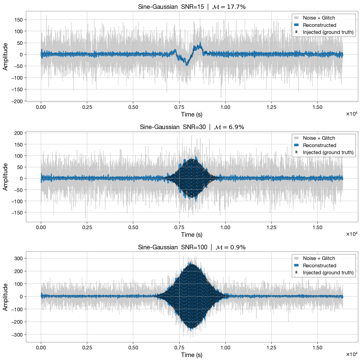
../_images/notebooks_training_tutorial_colab_14_0.png

Step 6 — Test on sine-Gaussian injections¶

We generate fresh test examples — PyCBC (numpy) noise with a sine-Gaussian injected at a range of SNRs — and run them through the trained model. The model was never trained on these specific examples. We use three different test examples at three different SNRs, reporting the SNR and mismatch (\(\mathcal{M}\)) above each plot. Intuitively, the model better recovers louder glitches than quieter ones. The reconstructions below feature high-frequency artifacts as the model training did not fully converge, and it is a reduced architecture compared to the published version. Improved performance can be achieved by training this model until convergence or by modifying the layers of DeepExtractor’s U-Net to the published architecture, and increasing the resolution of the STFT spectrograms (please see above).

[16]:

def reconstruct(noisy_signal, model, scaler, device, n_fft, hop_length, win_length):
    """Scale → STFT → U-Net → iSTFT → unscale → subtract background."""
    # Scale
    scaled = scaler.transform(noisy_signal.reshape(-1, 1)).reshape(noisy_signal.shape)

    # STFT
    window = torch.hann_window(win_length)
    t = torch.tensor(scaled, dtype=torch.float32).unsqueeze(0)  # (1, time)
    stft = torch.stft(t, n_fft=n_fft, hop_length=hop_length, win_length=win_length,
                      window=window, return_complex=True)
    mag   = torch.abs(stft)
    phase = torch.angle(stft)
    spec  = torch.stack([mag, phase], dim=1)  # (1, 2, F, T)

    # U-Net inference
    model.eval()
    with torch.no_grad():
        bg_spec = model(spec.to(device)).cpu()  # predicted background spectrogram

    # iSTFT
    bg_mag   = bg_spec[:, 0, :, :]
    bg_phase = bg_spec[:, 1, :, :]
    bg_complex = bg_mag * torch.exp(1j * bg_phase)
    bg_td = torch.istft(bg_complex, n_fft=n_fft, hop_length=hop_length,
                        win_length=win_length, window=window,
                        length=noisy_signal.shape[-1])

    # Unscale and subtract background to recover signal
    bg_unscaled = scaler.inverse_transform(bg_td.numpy().reshape(-1, 1)).reshape(-1)
    noisy_unscaled = noisy_signal.copy()
    reconstruction = noisy_unscaled - bg_unscaled
    return reconstruction

[39]:

T_INJ = T / 2
SNR_VALUES = [15, 30, 100]

def overlap(a, b):
    """Normalised time-domain overlap (match) between two real signals.
    Equivalent to the PyCBC match on whitened data (flat PSD)."""
    return np.dot(a, b) / np.sqrt(np.dot(a, a) * np.dot(b, b))

fig, axes = plt.subplots(len(SNR_VALUES), 1, figsize=(12, 4 * len(SNR_VALUES)))
t_axis = np.arange(LENGTH) * DT

for ax, snr in zip(axes, SNR_VALUES):
    noise = generate_gaussian_noise(mean, std_dev, 1, (LENGTH,), bilby_noise=False)[0]

    # We set freq_max=256 when generating the sine-Gaussians for visualization purposes. This can be increased to the Nyquist frequency (i.e. freq_max=2048).
    _, wavelet = generate_sine_gaussian(duration=0.5, freq_max=256)
    wavelet = wavelet - np.mean(wavelet)
    wavelet = whitened_snr_scaling(wavelet, snr=snr)

    len_glitch = len(wavelet)
    id_start   = int(T_INJ * SAMPLE_RATE) - len_glitch // 2
    noisy      = noise.copy()
    noisy[id_start : id_start + len_glitch] += wavelet

    injected = np.zeros(LENGTH)
    injected[id_start : id_start + len_glitch] = wavelet

    reconstructed = reconstruct(noisy, model, scaler, DEVICE, N_FFT, HOP_LENGTH, WIN_LENGTH)

    match    = overlap(injected, reconstructed)
    mismatch = 1.0 - match

    ax.plot(t_axis, noisy,         color="gray",  lw=0.8, alpha=0.4, label="Noise + Glitch")
    ax.plot(t_axis, reconstructed, color="C0",    lw=1.5, label="Reconstructed")
    ax.plot(t_axis, injected,      color="black", lw=1.5, alpha=0.6, linestyle="--", label="Injected (ground truth)")
    ax.set_title(
        f"Sine-Gaussian  SNR={snr}  |  "
        f"$\\mathcal{{M}} = {mismatch*100:.1f} \% $"
    )
    ax.set_xlabel("Time (s)")
    ax.set_ylabel("Amplitude")
    ax.legend(loc="upper right")
    ax.grid(True)

plt.tight_layout()
plt.show()

Generating pycbc noise...
Generating pycbc noise...
Generating pycbc noise...

../_images/notebooks_training_tutorial_colab_17_1.png

Part II — Hackathon Tasks¶

The tutorial above trained a baseline DeepExtractor (STFT U-Net) on synthetic data. Now try four targeted experiments — each changes one aspect of the pipeline. All tasks share the same fixed test set (generated below) so results are comparable.

Task	What you change	Key question
1	Number of U-Net encoder levels	How does model depth affect quality?
2	Model domain: STFT → 1-D time-domain	Does operating on raw waveforms help?
3	Training-set size `N_TRAIN`	How much data do we really need?
4	Synthetic training signal types	Does a diverse training set generalise better?

LISA / Mojito note — This tutorial runs at SAMPLE_RATE = 4096 Hz, T = 2 s, LENGTH = 8192. The Mojito LISA dataset uses dt = 2.0 s (0.5 Hz) with 1000-sample windows. For LISA-compatible parameters set SAMPLE_RATE = 0.5 and T = 16384.0 in the Configuration cell, re-run from the top, and adjust signal durations/frequencies (e.g. duration range 20–8000 s, freq_max = SAMPLE_RATE / 2 = 0.25 Hz).

[18]:

# --- Optional: install gengli for out-of-sample blip testing (Task 4) ----------
try:
    import gengli
    GENGLI_AVAILABLE = True
    print("gengli available.")
except ImportError:
    try:
        import subprocess, sys
        subprocess.check_call([sys.executable, "-m", "pip", "install", "gengli", "-q"])
        import gengli
        GENGLI_AVAILABLE = True
        print("gengli installed.")
    except Exception:
        GENGLI_AVAILABLE = False
        print("gengli not available — blip test in Task 4 will be skipped.")

# --- Fixed test set (sine-Gaussian injections at three SNRs) ------------------
# Seeded once; do NOT re-run this cell mid-session to keep comparisons fair.
import random as _random
_random.seed(42)
np.random.seed(42)
torch.manual_seed(42)

_N_PER_SNR  = 10
_SNR_VALS   = [15, 30, 100]
_T_INJ_TEST = T / 2

_noisy_buf, _inj_buf, _snr_buf = [], [], []
for _snr in _SNR_VALS:
    for _ in range(_N_PER_SNR):
        _n   = generate_gaussian_noise(mean, std_dev, 1, (LENGTH,), bilby_noise=False)[0]
        _, _w = generate_sine_gaussian(duration=0.5, freq_max=256)
        _w   = _w - np.mean(_w)
        _w   = whitened_snr_scaling(_w, snr=_snr)
        _L   = len(_w)
        _i0  = int(_T_INJ_TEST * SAMPLE_RATE) - _L // 2
        _nn  = _n.copy()
        _nn[_i0:_i0 + _L] += _w
        _ij  = np.zeros(LENGTH)
        _ij[_i0:_i0 + _L] = _w
        _noisy_buf.append(_nn)
        _inj_buf.append(_ij)
        _snr_buf.append(_snr)

TEST_NOISY    = np.array(_noisy_buf)    # (30, LENGTH)
TEST_INJECTED = np.array(_inj_buf)      # (30, LENGTH)
TEST_SNRS     = np.array(_snr_buf)
print(f"Fixed test set ready: {len(TEST_NOISY)} examples, SNRs = {_SNR_VALS}")

gengli available.
Generating pycbc noise...
Generating pycbc noise...
Generating pycbc noise...
Generating pycbc noise...
Generating pycbc noise...
Generating pycbc noise...
Generating pycbc noise...
Generating pycbc noise...
Generating pycbc noise...
Generating pycbc noise...
Generating pycbc noise...
Generating pycbc noise...
Generating pycbc noise...
Generating pycbc noise...
Generating pycbc noise...
Generating pycbc noise...
Generating pycbc noise...
Generating pycbc noise...
Generating pycbc noise...
Generating pycbc noise...
Generating pycbc noise...
Generating pycbc noise...
Generating pycbc noise...
Generating pycbc noise...
Generating pycbc noise...
Generating pycbc noise...
Generating pycbc noise...
Generating pycbc noise...
Generating pycbc noise...
Generating pycbc noise...
Fixed test set ready: 30 examples, SNRs = [15, 30, 100]

[19]:

# --- Shared helpers used by all four tasks ------------------------------------
EPOCHS_TASK = 20   # reduce to 10 for quicker runs; increase for better convergence


def _train_stft(mdl, tr_ld, vl_ld, epochs=EPOCHS_TASK):
    # Train an STFT model (or any model whose loader yields 2-D spectrograms).
    _lfn = nn.MSELoss()
    _opt = optim.Adam(mdl.parameters(), lr=LR)
    _sch = ReduceLROnPlateau(_opt, mode="min", factor=LR_FACTOR, patience=LR_PATIENCE)
    _amp = torch.amp.GradScaler("cuda") if DEVICE == "cuda" else torch.amp.GradScaler("cpu", enabled=False)
    tr_ls, vl_ls = [], []
    best_v, es_c = float("inf"), 0
    for ep in range(epochs):
        tl, _, _ = train_fn(tr_ld, mdl, "generic", _opt, _lfn, _amp, DEVICE)
        vl, _, _ = check_accuracy(vl_ld, mdl, "generic", device=DEVICE)
        tr_ls.append(tl)
        vl_ls.append(vl)
        _sch.step(vl)
        print(f"  ep {ep+1:>2}/{epochs}  train={tl:.5f}  val={vl:.5f}")
        if vl < best_v:
            best_v = vl
            es_c   = 0
        else:
            es_c += 1
            if es_c >= EARLY_STOPPING_PATIENCE:
                print(f"  Early stopping at epoch {ep+1}.")
                break
    return tr_ls, vl_ls


def _mismatch_stft(mdl, scl=None):
    # Mean mismatch of an STFT model on the fixed test set.
    if scl is None:
        scl = scaler
    mm = [
        1.0 - overlap(inj, reconstruct(noisy, mdl, scl, DEVICE, N_FFT, HOP_LENGTH, WIN_LENGTH))
        for noisy, inj in zip(TEST_NOISY, TEST_INJECTED)
    ]
    return float(np.mean(mm))


def _mismatch_1d(mdl, scl=None):
    # Mean mismatch of a 1-D time-domain model on the fixed test set.
    if scl is None:
        scl = scaler
    mdl.eval()
    mm = []
    with torch.no_grad():
        for noisy, inj in zip(TEST_NOISY, TEST_INJECTED):
            sc_in  = scl.transform(noisy.reshape(-1, 1)).reshape(1, 1, -1)
            inp    = torch.tensor(sc_in, dtype=torch.float32).to(DEVICE)
            out    = mdl(inp).cpu().numpy().squeeze()
            bg_raw = scl.inverse_transform(out.reshape(-1, 1)).reshape(-1)
            mm.append(1.0 - overlap(inj, noisy - bg_raw))
    mdl.train()
    return float(np.mean(mm))


def _plot_val_curves(loss_dict, title="Validation Loss"):
    fig, ax = plt.subplots(figsize=(8, 4))
    for lbl, (_, vl) in loss_dict.items():
        ax.plot(range(1, len(vl) + 1), vl, label=lbl)
    ax.set_xlabel("Epoch")
    ax.set_ylabel("MSE Loss")
    ax.set_title(title)
    ax.legend()
    ax.grid(True)
    plt.tight_layout()
    plt.show()

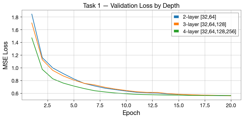
Task 1 — Effect of Model Depth¶

The baseline model uses features = [32, 64, 128, 256] (4 encoder levels). Shallower models train faster but may lack capacity; deeper ones risk overfitting on small datasets.

TODO: Run the comparison below as-is, then add a 5th level ([..., 512]) or strip it back to a single level and observe how the validation loss and test mismatch change.

Discussion questions:

At what depth does adding more layers stop helping?
Do you see signs of overfitting (val loss rising while train loss falls)?

[20]:

# --- Task 1: compare U-Net depths --------------------------------------------
# TODO: add or remove entries in features_configs to explore other depths
features_configs = {
    "2-layer [32,64]":           [32, 64],
    "3-layer [32,64,128]":       [32, 64, 128],
    "4-layer [32,64,128,256]":   [32, 64, 128, 256],   # matches baseline above
}

task1_curves    = {}   # label -> (train_losses, val_losses)
task1_mismatch  = {}   # label -> mean mismatch on TEST_NOISY

for lbl, feats in features_configs.items():
    print(f"\n{'─'*60}")
    print(f"Training: {lbl}  ({sum(p.numel() for p in UNET2D(2,2,feats).parameters()):,} params)")
    mdl = UNET2D(in_channels=2, out_channels=2, features=feats).to(DEVICE)
    tr_ls, vl_ls     = _train_stft(mdl, train_loader, val_loader)
    task1_curves[lbl]   = (tr_ls, vl_ls)
    task1_mismatch[lbl] = _mismatch_stft(mdl)
    print(f"  Mean test mismatch: {task1_mismatch[lbl]*100:.2f} %")

_plot_val_curves(task1_curves, title="Task 1 — Validation Loss by Depth")


────────────────────────────────────────────────────────────
Training: 2-layer [32,64]  (466,914 params)

Training on batch: 100%|██████████| 32/32 [00:07<00:00,  4.33it/s, loss=1.51]

Validation Loss: 1.842396
  ep  1/20  train=1.97619  val=1.84240

Training on batch: 100%|██████████| 32/32 [00:06<00:00,  4.66it/s, loss=1.18]

Validation Loss: 1.157481
  ep  2/20  train=1.32166  val=1.15748

Training on batch: 100%|██████████| 32/32 [00:06<00:00,  4.63it/s, loss=0.946]

Validation Loss: 0.996087
  ep  3/20  train=1.07190  val=0.99609

Training on batch: 100%|██████████| 32/32 [00:06<00:00,  4.64it/s, loss=0.855]

Validation Loss: 0.906955
  ep  4/20  train=0.94157  val=0.90695

Training on batch: 100%|██████████| 32/32 [00:06<00:00,  4.64it/s, loss=0.803]

Validation Loss: 0.824616
  ep  5/20  train=0.85367  val=0.82462

Training on batch: 100%|██████████| 32/32 [00:06<00:00,  4.63it/s, loss=0.784]

Validation Loss: 0.752851
  ep  6/20  train=0.78944  val=0.75285

Training on batch: 100%|██████████| 32/32 [00:06<00:00,  4.61it/s, loss=0.642]

Validation Loss: 0.712364
  ep  7/20  train=0.74076  val=0.71236

Training on batch: 100%|██████████| 32/32 [00:06<00:00,  4.62it/s, loss=0.809]

Validation Loss: 0.676749
  ep  8/20  train=0.70887  val=0.67675

Training on batch: 100%|██████████| 32/32 [00:06<00:00,  4.61it/s, loss=0.646]

Validation Loss: 0.654356
  ep  9/20  train=0.67910  val=0.65436

Training on batch: 100%|██████████| 32/32 [00:06<00:00,  4.62it/s, loss=0.75]

Validation Loss: 0.631869
  ep 10/20  train=0.66177  val=0.63187

Training on batch: 100%|██████████| 32/32 [00:06<00:00,  4.61it/s, loss=0.551]

Validation Loss: 0.612898
  ep 11/20  train=0.63885  val=0.61290

Training on batch: 100%|██████████| 32/32 [00:07<00:00,  4.49it/s, loss=0.799]

Validation Loss: 0.606133
  ep 12/20  train=0.63187  val=0.60613

Training on batch: 100%|██████████| 32/32 [00:06<00:00,  4.59it/s, loss=0.436]

Validation Loss: 0.597395
  ep 13/20  train=0.61334  val=0.59740

Training on batch: 100%|██████████| 32/32 [00:07<00:00,  4.54it/s, loss=0.551]

Validation Loss: 0.585908
  ep 14/20  train=0.60663  val=0.58591

Training on batch: 100%|██████████| 32/32 [00:06<00:00,  4.58it/s, loss=0.44]

Validation Loss: 0.579648
  ep 15/20  train=0.59667  val=0.57965

Training on batch: 100%|██████████| 32/32 [00:07<00:00,  4.54it/s, loss=0.603]

Validation Loss: 0.572915
  ep 16/20  train=0.59427  val=0.57292

Training on batch: 100%|██████████| 32/32 [00:07<00:00,  4.54it/s, loss=0.512]

Validation Loss: 0.569668
  ep 17/20  train=0.58693  val=0.56967

Training on batch: 100%|██████████| 32/32 [00:07<00:00,  4.55it/s, loss=0.569]

Validation Loss: 0.564380
  ep 18/20  train=0.58305  val=0.56438

Training on batch: 100%|██████████| 32/32 [00:07<00:00,  4.53it/s, loss=0.69]

Validation Loss: 0.559508
  ep 19/20  train=0.58168  val=0.55951

Training on batch: 100%|██████████| 32/32 [00:07<00:00,  4.52it/s, loss=0.564]

Validation Loss: 0.558261
  ep 20/20  train=0.57570  val=0.55826
  Mean test mismatch: 15.62 %

────────────────────────────────────────────────────────────
Training: 3-layer [32,64,128]  (1,926,754 params)

Training on batch: 100%|██████████| 32/32 [00:08<00:00,  3.57it/s, loss=1.48]

Validation Loss: 1.703437
  ep  1/20  train=1.86348  val=1.70344

Training on batch: 100%|██████████| 32/32 [00:09<00:00,  3.40it/s, loss=1.25]

Validation Loss: 1.126283
  ep  2/20  train=1.28804  val=1.12628

Training on batch: 100%|██████████| 32/32 [00:09<00:00,  3.26it/s, loss=1.08]

Validation Loss: 0.957577
  ep  3/20  train=1.05792  val=0.95758

Training on batch: 100%|██████████| 32/32 [00:11<00:00,  2.85it/s, loss=0.853]

Validation Loss: 0.869897
  ep  4/20  train=0.92894  val=0.86990

Training on batch: 100%|██████████| 32/32 [00:10<00:00,  3.00it/s, loss=0.845]

Validation Loss: 0.805657
  ep  5/20  train=0.84751  val=0.80566

Training on batch: 100%|██████████| 32/32 [00:11<00:00,  2.82it/s, loss=0.669]

Validation Loss: 0.753861
  ep  6/20  train=0.78284  val=0.75386

Training on batch: 100%|██████████| 32/32 [00:10<00:00,  2.91it/s, loss=0.794]

Validation Loss: 0.728559
  ep  7/20  train=0.74295  val=0.72856

Training on batch: 100%|██████████| 32/32 [00:10<00:00,  2.95it/s, loss=0.757]

Validation Loss: 0.690626
  ep  8/20  train=0.72155  val=0.69063

Training on batch: 100%|██████████| 32/32 [00:11<00:00,  2.72it/s, loss=0.67]

Validation Loss: 0.662885
  ep  9/20  train=0.68957  val=0.66288

Training on batch: 100%|██████████| 32/32 [00:10<00:00,  2.94it/s, loss=0.701]

Validation Loss: 0.640880
  ep 10/20  train=0.66697  val=0.64088

Training on batch: 100%|██████████| 32/32 [00:10<00:00,  2.93it/s, loss=0.549]

Validation Loss: 0.621393
  ep 11/20  train=0.64634  val=0.62139

Training on batch: 100%|██████████| 32/32 [00:10<00:00,  3.12it/s, loss=0.601]

Validation Loss: 0.611121
  ep 12/20  train=0.63411  val=0.61112

Training on batch: 100%|██████████| 32/32 [00:10<00:00,  3.12it/s, loss=0.742]

Validation Loss: 0.610201
  ep 13/20  train=0.62542  val=0.61020

Training on batch: 100%|██████████| 32/32 [00:10<00:00,  3.09it/s, loss=0.717]

Validation Loss: 0.591952
  ep 14/20  train=0.61739  val=0.59195

Training on batch: 100%|██████████| 32/32 [00:10<00:00,  3.10it/s, loss=0.602]

Validation Loss: 0.581212
  ep 15/20  train=0.60427  val=0.58121

Training on batch: 100%|██████████| 32/32 [00:10<00:00,  3.12it/s, loss=0.647]

Validation Loss: 0.575712
  ep 16/20  train=0.59778  val=0.57571

Training on batch: 100%|██████████| 32/32 [00:10<00:00,  3.12it/s, loss=0.641]

Validation Loss: 0.569919
  ep 17/20  train=0.59165  val=0.56992

Training on batch: 100%|██████████| 32/32 [00:10<00:00,  3.13it/s, loss=0.668]

Validation Loss: 0.566680
  ep 18/20  train=0.58754  val=0.56668

Training on batch: 100%|██████████| 32/32 [00:10<00:00,  3.12it/s, loss=0.506]

Validation Loss: 0.563145
  ep 19/20  train=0.57907  val=0.56314

Training on batch: 100%|██████████| 32/32 [00:10<00:00,  3.08it/s, loss=0.599]

Validation Loss: 0.558316
  ep 20/20  train=0.57666  val=0.55832
  Mean test mismatch: 14.22 %

────────────────────────────────────────────────────────────
Training: 4-layer [32,64,128,256]  (7,762,786 params)

Training on batch: 100%|██████████| 32/32 [00:13<00:00,  2.45it/s, loss=1.31]

Validation Loss: 1.468930
  ep  1/20  train=1.61191  val=1.46893

Training on batch: 100%|██████████| 32/32 [00:12<00:00,  2.50it/s, loss=0.943]

Validation Loss: 0.973738
  ep  2/20  train=1.07422  val=0.97374

Training on batch: 100%|██████████| 32/32 [00:12<00:00,  2.47it/s, loss=0.796]

Validation Loss: 0.825409
  ep  3/20  train=0.88673  val=0.82541

Training on batch: 100%|██████████| 32/32 [00:13<00:00,  2.41it/s, loss=0.843]

Validation Loss: 0.757717
  ep  4/20  train=0.79567  val=0.75772

Training on batch: 100%|██████████| 32/32 [00:13<00:00,  2.41it/s, loss=0.712]

Validation Loss: 0.711353
  ep  5/20  train=0.73683  val=0.71135

Training on batch: 100%|██████████| 32/32 [00:13<00:00,  2.41it/s, loss=0.77]

Validation Loss: 0.671415
  ep  6/20  train=0.69860  val=0.67141

Training on batch: 100%|██████████| 32/32 [00:13<00:00,  2.40it/s, loss=0.657]

Validation Loss: 0.637529
  ep  7/20  train=0.66571  val=0.63753

Training on batch: 100%|██████████| 32/32 [00:12<00:00,  2.48it/s, loss=0.781]

Validation Loss: 0.617889
  ep  8/20  train=0.64511  val=0.61789

Training on batch: 100%|██████████| 32/32 [00:12<00:00,  2.50it/s, loss=0.771]

Validation Loss: 0.601279
  ep  9/20  train=0.62528  val=0.60128

Training on batch: 100%|██████████| 32/32 [00:12<00:00,  2.52it/s, loss=0.602]

Validation Loss: 0.589714
  ep 10/20  train=0.60662  val=0.58971

Training on batch: 100%|██████████| 32/32 [00:12<00:00,  2.52it/s, loss=0.81]

Validation Loss: 0.580445
  ep 11/20  train=0.59909  val=0.58045

Training on batch: 100%|██████████| 32/32 [00:12<00:00,  2.52it/s, loss=0.53]

Validation Loss: 0.575858
  ep 12/20  train=0.58321  val=0.57586

Training on batch: 100%|██████████| 32/32 [00:12<00:00,  2.52it/s, loss=0.553]

Validation Loss: 0.572049
  ep 13/20  train=0.57363  val=0.57205

Training on batch: 100%|██████████| 32/32 [00:12<00:00,  2.53it/s, loss=0.646]

Validation Loss: 0.569053
  ep 14/20  train=0.56754  val=0.56905

Training on batch: 100%|██████████| 32/32 [00:12<00:00,  2.53it/s, loss=0.496]

Validation Loss: 0.568510
  ep 15/20  train=0.55768  val=0.56851

Training on batch: 100%|██████████| 32/32 [00:12<00:00,  2.52it/s, loss=0.476]

Validation Loss: 0.563967
  ep 16/20  train=0.54936  val=0.56397

Training on batch: 100%|██████████| 32/32 [00:12<00:00,  2.52it/s, loss=0.666]

Validation Loss: 0.562845
  ep 17/20  train=0.54721  val=0.56284

Training on batch: 100%|██████████| 32/32 [00:12<00:00,  2.52it/s, loss=0.555]

Validation Loss: 0.561657
  ep 18/20  train=0.53844  val=0.56166

Training on batch: 100%|██████████| 32/32 [00:12<00:00,  2.52it/s, loss=0.525]

Validation Loss: 0.562531
  ep 19/20  train=0.53070  val=0.56253

Training on batch: 100%|██████████| 32/32 [00:12<00:00,  2.50it/s, loss=0.527]

Validation Loss: 0.562766
  ep 20/20  train=0.52310  val=0.56277
  Mean test mismatch: 11.78 %

../_images/notebooks_training_tutorial_colab_22_121.png

[21]:

# Task 1 summary bar chart
fig, ax = plt.subplots(figsize=(7, 4))
lbls = list(task1_mismatch.keys())
vals = [task1_mismatch[l] * 100 for l in lbls]
ax.bar(lbls, vals, color="C0")
ax.set_ylabel("Mean Mismatch (%)")
ax.set_title("Task 1 — Mismatch vs. Model Depth")
ax.tick_params(axis="x", labelrotation=15)
ax.grid(axis="y")
plt.tight_layout()
plt.show()
for l, v in zip(lbls, vals):
    print(f"  {l}: {v:.2f} %")

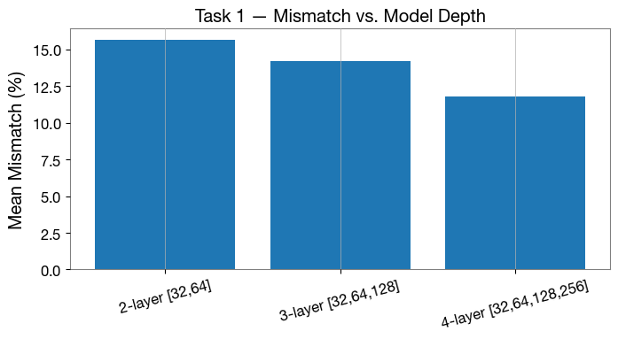
../_images/notebooks_training_tutorial_colab_23_0.png

  2-layer [32,64]: 15.62 %
  3-layer [32,64,128]: 14.22 %
  4-layer [32,64,128,256]: 11.78 %

Task 2 — Time-Domain vs. STFT Model¶

DeepExtractor normally operates on STFT spectrograms (magnitude + phase, shape (2, 129, 129)). UNET1D instead processes the raw 1-D waveform directly — no frequency transform.

	Input shape	Ops	Params (same depth)
`UNET2D` (STFT)	`(B, 2, 129, 129)`	2-D convolutions	~7 M
`UNET1D` (TD)	`(B, 1, 8192)`	1-D convolutions	~3 M

TODO: Run the cells below to train the 1-D model, then compare its mismatch against the STFT baseline.

Discussion questions:

Which model achieves lower mismatch?
Is the time-domain model faster or slower to train per epoch?
What information does the STFT representation preserve that the time domain does not?

[22]:

# --- Task 2: 1-D DataLoaders (reuse already-scaled arrays) -------------------
from deepextractor.models.architectures import UNET1D

# Add a channel dimension: (N, LENGTH) -> (N, 1, LENGTH)
x_tr_1d = torch.tensor(glitch_train_scaled, dtype=torch.float32).unsqueeze(1)
y_tr_1d = torch.tensor(bg_train_scaled,     dtype=torch.float32).unsqueeze(1)
x_vl_1d = torch.tensor(glitch_val_scaled,   dtype=torch.float32).unsqueeze(1)
y_vl_1d = torch.tensor(bg_val_scaled,       dtype=torch.float32).unsqueeze(1)

train_ds_1d     = TensorDataset(x_tr_1d, y_tr_1d)
val_ds_1d       = TensorDataset(x_vl_1d, y_vl_1d)
train_loader_1d = DataLoader(train_ds_1d, batch_size=BATCH_SIZE, shuffle=True)
val_loader_1d   = DataLoader(val_ds_1d,   batch_size=BATCH_SIZE, shuffle=False)
print(f"1-D input shape: {x_tr_1d.shape}")

1-D input shape: torch.Size([1000, 1, 8192])

[23]:

# --- Task 2: train UNET1D and compare with STFT baseline --------------------
model_1d = UNET1D(in_channels=1, out_channels=1, features=[32, 64, 128, 256]).to(DEVICE)
print(f"UNET1D parameters: {sum(p.numel() for p in model_1d.parameters()):,}")

print("\nTraining UNET1D (time-domain)...")
trl_1d, vll_1d = _train_stft(model_1d, train_loader_1d, val_loader_1d)
mm_1d = _mismatch_1d(model_1d)
print(f"\nUNET1D  mean test mismatch : {mm_1d*100:.2f} %")

# Retrieve STFT result from Task 1 (4-layer) or re-evaluate the baseline
_stft_lbl = "4-layer [32,64,128,256]"
mm_stft   = task1_mismatch.get(_stft_lbl, _mismatch_stft(model))
print(f"UNET2D  mean test mismatch : {mm_stft*100:.2f} %")

UNET1D parameters: 2,707,809

Training UNET1D (time-domain)...

Training on batch: 100%|██████████| 32/32 [00:17<00:00,  1.83it/s, loss=0.0364]

Validation Loss: 0.030803
  ep  1/20  train=0.05326  val=0.03080

Training on batch: 100%|██████████| 32/32 [00:14<00:00,  2.24it/s, loss=0.0262]

Validation Loss: 0.025569
  ep  2/20  train=0.02853  val=0.02557

Training on batch: 100%|██████████| 32/32 [00:14<00:00,  2.24it/s, loss=0.024]

Validation Loss: 0.023037
  ep  3/20  train=0.02465  val=0.02304

Training on batch: 100%|██████████| 32/32 [00:14<00:00,  2.28it/s, loss=0.0198]

Validation Loss: 0.021752
  ep  4/20  train=0.02283  val=0.02175

Training on batch: 100%|██████████| 32/32 [00:14<00:00,  2.28it/s, loss=0.021]

Validation Loss: 0.020767
  ep  5/20  train=0.02180  val=0.02077

Training on batch: 100%|██████████| 32/32 [00:14<00:00,  2.28it/s, loss=0.0215]

Validation Loss: 0.020052
  ep  6/20  train=0.02105  val=0.02005

Training on batch: 100%|██████████| 32/32 [00:14<00:00,  2.28it/s, loss=0.0205]

Validation Loss: 0.019577
  ep  7/20  train=0.02046  val=0.01958

Training on batch: 100%|██████████| 32/32 [00:14<00:00,  2.23it/s, loss=0.0209]

Validation Loss: 0.019066
  ep  8/20  train=0.01996  val=0.01907

Training on batch: 100%|██████████| 32/32 [00:14<00:00,  2.25it/s, loss=0.0179]

Validation Loss: 0.018676
  ep  9/20  train=0.01950  val=0.01868

Training on batch: 100%|██████████| 32/32 [00:14<00:00,  2.23it/s, loss=0.022]

Validation Loss: 0.018241
  ep 10/20  train=0.01921  val=0.01824

Training on batch: 100%|██████████| 32/32 [00:14<00:00,  2.21it/s, loss=0.0192]

Validation Loss: 0.017972
  ep 11/20  train=0.01883  val=0.01797

Training on batch: 100%|██████████| 32/32 [00:14<00:00,  2.25it/s, loss=0.0159]

Validation Loss: 0.017709
  ep 12/20  train=0.01841  val=0.01771

Training on batch: 100%|██████████| 32/32 [00:14<00:00,  2.23it/s, loss=0.021]

Validation Loss: 0.017410
  ep 13/20  train=0.01823  val=0.01741

Training on batch: 100%|██████████| 32/32 [00:14<00:00,  2.24it/s, loss=0.0164]

Validation Loss: 0.017166
  ep 14/20  train=0.01787  val=0.01717

Training on batch: 100%|██████████| 32/32 [00:14<00:00,  2.23it/s, loss=0.0172]

Validation Loss: 0.016972
  ep 15/20  train=0.01768  val=0.01697

Training on batch: 100%|██████████| 32/32 [00:14<00:00,  2.19it/s, loss=0.0134]

Validation Loss: 0.016779
  ep 16/20  train=0.01738  val=0.01678

Training on batch: 100%|██████████| 32/32 [00:14<00:00,  2.20it/s, loss=0.0169]

Validation Loss: 0.016555
  ep 17/20  train=0.01725  val=0.01655

Training on batch: 100%|██████████| 32/32 [00:14<00:00,  2.20it/s, loss=0.0175]

Validation Loss: 0.016353
  ep 18/20  train=0.01705  val=0.01635

Training on batch: 100%|██████████| 32/32 [00:14<00:00,  2.18it/s, loss=0.0175]

Validation Loss: 0.016186
  ep 19/20  train=0.01686  val=0.01619

Training on batch: 100%|██████████| 32/32 [00:15<00:00,  2.08it/s, loss=0.0188]

Validation Loss: 0.016031
  ep 20/20  train=0.01671  val=0.01603

UNET1D  mean test mismatch : 25.59 %
UNET2D  mean test mismatch : 11.78 %

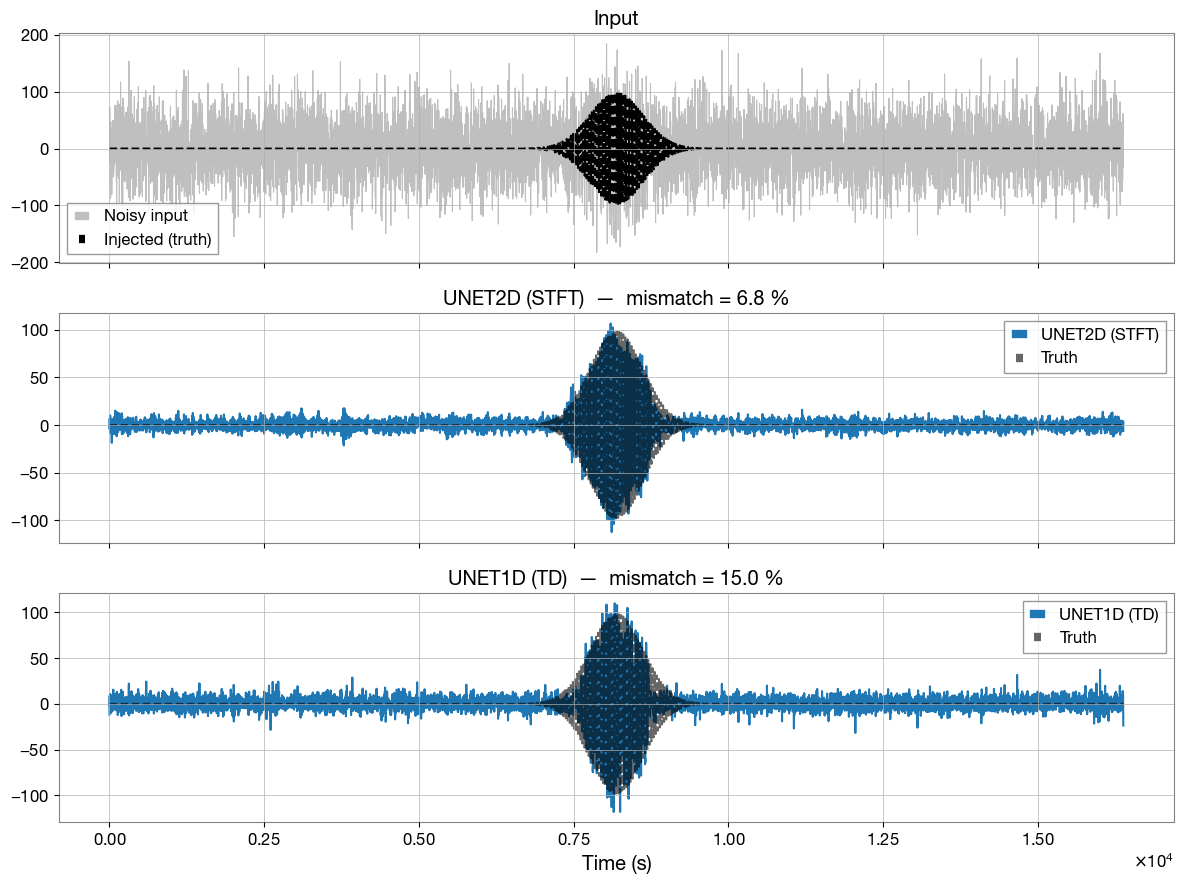
[40]:

# Task 2: side-by-side reconstruction at SNR=30 for one test example
_idx    = int(np.where(TEST_SNRS == 30)[0][0])
_noisy  = TEST_NOISY[_idx]
_inj    = TEST_INJECTED[_idx]
t_axis  = np.arange(LENGTH) * DT

_r_stft = reconstruct(_noisy, model, scaler, DEVICE, N_FFT, HOP_LENGTH, WIN_LENGTH)

model_1d.eval()
with torch.no_grad():
    _sc  = scaler.transform(_noisy.reshape(-1, 1)).reshape(1, 1, -1)
    _out = model_1d(torch.tensor(_sc, dtype=torch.float32).to(DEVICE)).cpu().numpy().squeeze()
    _bg  = scaler.inverse_transform(_out.reshape(-1, 1)).reshape(-1)
_r_1d = _noisy - _bg

fig, axes = plt.subplots(3, 1, figsize=(12, 9), sharex=True)

axes[0].plot(t_axis, _noisy, color="gray", lw=0.8, alpha=0.5, label="Noisy input")
axes[0].plot(t_axis, _inj,  color="black", lw=1.5, ls="--", label="Injected (truth)")
axes[0].set_title("Input")
axes[0].legend(); axes[0].grid(True)

for ax, recon, lbl in [(axes[1], _r_stft, "UNET2D (STFT)"),
                       (axes[2], _r_1d,   "UNET1D (TD)")]:
    mm = 1.0 - overlap(_inj, recon)
    ax.plot(t_axis, recon, lw=1.5, label=lbl)
    ax.plot(t_axis, _inj, color="black", lw=1.5, ls="--", alpha=0.6, label="Truth")
    ax.set_title(f"{lbl}  —  mismatch = {mm*100:.1f} %")
    ax.legend(); ax.grid(True)

axes[-1].set_xlabel("Time (s)")
plt.tight_layout()
plt.show()

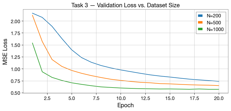
../_images/notebooks_training_tutorial_colab_27_0.png

Task 3 — Effect of Dataset Size¶

More training data usually improves generalisation — but generating (or labelling) data has a cost. Here you train the same model architecture on datasets of increasing size and measure how reconstruction quality on the fixed test set changes.

TODO: Run the cell below, then add larger values like 2000 or 5000 to n_train_values.

Discussion questions:

Is there a “knee” in the mismatch-vs-N curve after which more data stops helping?
What does this imply about how much real detector data you would need?

[25]:

# --- Task 3: vary training-set size ------------------------------------------
# TODO: add more values (e.g. 2000, 5000) to see the full curve
n_train_values = [200, 500, 1000]

task3_curves   = {}
task3_mismatch = {}

for n_tr in n_train_values:
    print(f"\n{'─'*60}\nN_TRAIN = {n_tr}")

    _tr_noise = generate_gaussian_noise(mean, std_dev, n_tr,  (LENGTH,), bilby_noise=False)
    _vl_noise = generate_gaussian_noise(mean, std_dev, N_VAL, (LENGTH,), bilby_noise=False)
    _gl_tr, _bg_tr = generate_synthetic_data(_tr_noise, bilby_noise=False, phase="train")
    _gl_vl, _bg_vl = generate_synthetic_data(_vl_noise, bilby_noise=False, phase="val")

    _sc_gl_tr  = scaler.transform(_gl_tr.reshape(-1, 1)).reshape(_gl_tr.shape)
    _sc_bg_tr  = scaler.transform(_bg_tr.reshape(-1, 1)).reshape(_bg_tr.shape)
    _sc_gl_vl  = scaler.transform(_gl_vl.reshape(-1, 1)).reshape(_gl_vl.shape)
    _sc_bg_vl  = scaler.transform(_bg_vl.reshape(-1, 1)).reshape(_bg_vl.shape)

    _sp_gl_tr  = to_mag_phase(_sc_gl_tr)
    _sp_bg_tr  = to_mag_phase(_sc_bg_tr)
    _sp_gl_vl  = to_mag_phase(_sc_gl_vl)
    _sp_bg_vl  = to_mag_phase(_sc_bg_vl)

    _ld_tr = DataLoader(TensorDataset(_sp_gl_tr, _sp_bg_tr), batch_size=BATCH_SIZE, shuffle=True)
    _ld_vl = DataLoader(TensorDataset(_sp_gl_vl, _sp_bg_vl), batch_size=BATCH_SIZE, shuffle=False)

    _mdl = UNET2D(in_channels=2, out_channels=2, features=[32, 64, 128, 256]).to(DEVICE)
    tr_ls, vl_ls           = _train_stft(_mdl, _ld_tr, _ld_vl)
    task3_curves[f"N={n_tr}"]   = (tr_ls, vl_ls)
    task3_mismatch[f"N={n_tr}"] = _mismatch_stft(_mdl)
    print(f"  Mean test mismatch: {task3_mismatch[f'N={n_tr}']*100:.2f} %")

_plot_val_curves(task3_curves, title="Task 3 — Validation Loss vs. Dataset Size")


────────────────────────────────────────────────────────────
N_TRAIN = 200
Generating pycbc noise...
Generating pycbc noise...

Generating Synthetic Train Data:   0%|          | 0/200 [00:00<?, ?it/s]/Users/tomdooney/Documents/Work/Projects/deepextractor/src/deepextractor/utils/signal.py:12: RuntimeWarning: divide by zero encountered in divide
  glitch = (glitch.T * snr / np.sqrt(true_sigma_sq)).T
Generating Synthetic Train Data: 100%|██████████| 200/200 [00:00<00:00, 287.47it/s]
Generating Synthetic Val Data: 100%|██████████| 200/200 [00:00<00:00, 327.09it/s]
Training on batch: 100%|██████████| 7/7 [00:03<00:00,  1.75it/s, loss=1.89]

Validation Loss: 2.160550
  ep  1/20  train=1.99924  val=2.16055

Training on batch: 100%|██████████| 7/7 [00:02<00:00,  2.47it/s, loss=1.71]

Validation Loss: 2.072416
  ep  2/20  train=1.78770  val=2.07242

Training on batch: 100%|██████████| 7/7 [00:02<00:00,  2.59it/s, loss=1.5]

Validation Loss: 1.885873
  ep  3/20  train=1.59588  val=1.88587

Training on batch: 100%|██████████| 7/7 [00:02<00:00,  2.64it/s, loss=1.36]

Validation Loss: 1.631024
  ep  4/20  train=1.43213  val=1.63102

Training on batch: 100%|██████████| 7/7 [00:02<00:00,  2.54it/s, loss=1.27]

Validation Loss: 1.396365
  ep  5/20  train=1.30827  val=1.39637

Training on batch: 100%|██████████| 7/7 [00:02<00:00,  2.65it/s, loss=1.19]

Validation Loss: 1.234589
  ep  6/20  train=1.21598  val=1.23459

Training on batch: 100%|██████████| 7/7 [00:02<00:00,  2.62it/s, loss=1.04]

Validation Loss: 1.135841
  ep  7/20  train=1.13612  val=1.13584

Training on batch: 100%|██████████| 7/7 [00:02<00:00,  2.61it/s, loss=1.06]

Validation Loss: 1.067949
  ep  8/20  train=1.08583  val=1.06795

Training on batch: 100%|██████████| 7/7 [00:02<00:00,  2.61it/s, loss=1.01]

Validation Loss: 1.017442
  ep  9/20  train=1.03501  val=1.01744

Training on batch: 100%|██████████| 7/7 [00:02<00:00,  2.59it/s, loss=0.972]

Validation Loss: 0.975970
  ep 10/20  train=0.99106  val=0.97597

Training on batch: 100%|██████████| 7/7 [00:02<00:00,  2.57it/s, loss=0.864]

Validation Loss: 0.940768
  ep 11/20  train=0.94303  val=0.94077

Training on batch: 100%|██████████| 7/7 [00:02<00:00,  2.59it/s, loss=0.919]

Validation Loss: 0.905672
  ep 12/20  train=0.91649  val=0.90567

Training on batch: 100%|██████████| 7/7 [00:02<00:00,  2.60it/s, loss=0.92]

Validation Loss: 0.873171
  ep 13/20  train=0.88812  val=0.87317

Training on batch: 100%|██████████| 7/7 [00:02<00:00,  2.61it/s, loss=0.866]

Validation Loss: 0.848124
  ep 14/20  train=0.85629  val=0.84812

Training on batch: 100%|██████████| 7/7 [00:02<00:00,  2.61it/s, loss=0.877]

Validation Loss: 0.827886
  ep 15/20  train=0.83473  val=0.82789

Training on batch: 100%|██████████| 7/7 [00:02<00:00,  2.55it/s, loss=0.946]

Validation Loss: 0.805107
  ep 16/20  train=0.82308  val=0.80511

Training on batch: 100%|██████████| 7/7 [00:02<00:00,  2.61it/s, loss=0.788]

Validation Loss: 0.783462
  ep 17/20  train=0.78632  val=0.78346

Training on batch: 100%|██████████| 7/7 [00:02<00:00,  2.63it/s, loss=0.854]

Validation Loss: 0.768348
  ep 18/20  train=0.77741  val=0.76835

Training on batch: 100%|██████████| 7/7 [00:02<00:00,  2.59it/s, loss=0.77]

Validation Loss: 0.753309
  ep 19/20  train=0.75257  val=0.75331

Training on batch: 100%|██████████| 7/7 [00:02<00:00,  2.62it/s, loss=0.758]

Validation Loss: 0.738644
  ep 20/20  train=0.73729  val=0.73864
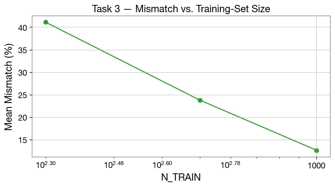
  Mean test mismatch: 41.09 %

────────────────────────────────────────────────────────────
N_TRAIN = 500
Generating pycbc noise...
Generating pycbc noise...

Generating Synthetic Train Data: 100%|██████████| 500/500 [00:01<00:00, 309.59it/s]
Generating Synthetic Val Data: 100%|██████████| 200/200 [00:00<00:00, 332.01it/s]
Training on batch: 100%|██████████| 16/16 [00:07<00:00,  2.10it/s, loss=1.71]

Validation Loss: 2.117698
  ep  1/20  train=1.89659  val=2.11770

Training on batch: 100%|██████████| 16/16 [00:07<00:00,  2.20it/s, loss=1.38]

Validation Loss: 1.569900
  ep  2/20  train=1.50604  val=1.56990

Training on batch: 100%|██████████| 16/16 [00:06<00:00,  2.29it/s, loss=1.17]

Validation Loss: 1.192910
  ep  3/20  train=1.23524  val=1.19291

Training on batch: 100%|██████████| 16/16 [00:06<00:00,  2.38it/s, loss=1.07]

Validation Loss: 1.049441
  ep  4/20  train=1.08950  val=1.04944

Training on batch: 100%|██████████| 16/16 [00:06<00:00,  2.42it/s, loss=1.03]

Validation Loss: 0.965502
  ep  5/20  train=0.99572  val=0.96550

Training on batch: 100%|██████████| 16/16 [00:26<00:00,  1.63s/it, loss=0.855]

Validation Loss: 0.906044
  ep  6/20  train=0.91969  val=0.90604

Training on batch: 100%|██████████| 16/16 [00:26<00:00,  1.65s/it, loss=0.855]

Validation Loss: 0.857629
  ep  7/20  train=0.86205  val=0.85763

Training on batch: 100%|██████████| 16/16 [00:05<00:00,  3.12it/s, loss=0.864]

Validation Loss: 0.817400
  ep  8/20  train=0.81676  val=0.81740

Training on batch: 100%|██████████| 16/16 [00:05<00:00,  3.08it/s, loss=0.806]

Validation Loss: 0.781027
  ep  9/20  train=0.78038  val=0.78103

Training on batch: 100%|██████████| 16/16 [00:05<00:00,  3.17it/s, loss=0.725]

Validation Loss: 0.757203
  ep 10/20  train=0.75056  val=0.75720

Training on batch: 100%|██████████| 16/16 [00:05<00:00,  3.15it/s, loss=0.702]

Validation Loss: 0.736130
  ep 11/20  train=0.72673  val=0.73613

Training on batch: 100%|██████████| 16/16 [00:05<00:00,  3.17it/s, loss=0.742]

Validation Loss: 0.717463
  ep 12/20  train=0.70778  val=0.71746

Training on batch: 100%|██████████| 16/16 [00:05<00:00,  3.10it/s, loss=0.655]

Validation Loss: 0.707719
  ep 13/20  train=0.68813  val=0.70772

Training on batch: 100%|██████████| 16/16 [00:05<00:00,  3.04it/s, loss=0.727]

Validation Loss: 0.690482
  ep 14/20  train=0.67351  val=0.69048

Training on batch: 100%|██████████| 16/16 [00:05<00:00,  2.95it/s, loss=0.677]

Validation Loss: 0.685018
  ep 15/20  train=0.65878  val=0.68502

Training on batch: 100%|██████████| 16/16 [00:05<00:00,  2.94it/s, loss=0.685]

Validation Loss: 0.675252
  ep 16/20  train=0.64500  val=0.67525

Training on batch: 100%|██████████| 16/16 [00:05<00:00,  2.86it/s, loss=0.593]

Validation Loss: 0.666552
  ep 17/20  train=0.62995  val=0.66655

Training on batch: 100%|██████████| 16/16 [00:05<00:00,  2.71it/s, loss=0.61]

Validation Loss: 0.660652
  ep 18/20  train=0.61888  val=0.66065

Training on batch: 100%|██████████| 16/16 [00:05<00:00,  2.68it/s, loss=0.579]

Validation Loss: 0.657312
  ep 19/20  train=0.60786  val=0.65731

Training on batch: 100%|██████████| 16/16 [00:06<00:00,  2.55it/s, loss=0.629]

Validation Loss: 0.648755
  ep 20/20  train=0.59984  val=0.64875
  Mean test mismatch: 23.76 %

────────────────────────────────────────────────────────────
N_TRAIN = 1000
Generating pycbc noise...
Generating pycbc noise...

Generating Synthetic Train Data: 100%|██████████| 1000/1000 [00:03<00:00, 263.64it/s]
Generating Synthetic Val Data: 100%|██████████| 200/200 [00:00<00:00, 269.44it/s]
Training on batch: 100%|██████████| 32/32 [00:14<00:00,  2.22it/s, loss=1.33]

Validation Loss: 1.537146
  ep  1/20  train=1.69460  val=1.53715

Training on batch: 100%|██████████| 32/32 [00:15<00:00,  2.01it/s, loss=1.01]

Validation Loss: 0.937342
  ep  2/20  train=1.07301  val=0.93734

Training on batch: 100%|██████████| 32/32 [00:15<00:00,  2.06it/s, loss=0.77]

Validation Loss: 0.820047
  ep  3/20  train=0.86895  val=0.82005

Training on batch: 100%|██████████| 32/32 [00:16<00:00,  1.97it/s, loss=0.751]

Validation Loss: 0.756323
  ep  4/20  train=0.78448  val=0.75632

Training on batch: 100%|██████████| 32/32 [00:16<00:00,  1.97it/s, loss=0.773]

Validation Loss: 0.707214
  ep  5/20  train=0.73424  val=0.70721

Training on batch: 100%|██████████| 32/32 [00:16<00:00,  2.00it/s, loss=0.705]

Validation Loss: 0.675107
  ep  6/20  train=0.69418  val=0.67511

Training on batch: 100%|██████████| 32/32 [00:14<00:00,  2.20it/s, loss=0.514]

Validation Loss: 0.646348
  ep  7/20  train=0.65893  val=0.64635

Training on batch: 100%|██████████| 32/32 [00:14<00:00,  2.25it/s, loss=0.673]

Validation Loss: 0.622028
  ep  8/20  train=0.64022  val=0.62203

Training on batch: 100%|██████████| 32/32 [00:13<00:00,  2.31it/s, loss=0.48]

Validation Loss: 0.610421
  ep  9/20  train=0.61766  val=0.61042

Training on batch: 100%|██████████| 32/32 [00:13<00:00,  2.34it/s, loss=0.567]

Validation Loss: 0.598711
  ep 10/20  train=0.60561  val=0.59871

Training on batch: 100%|██████████| 32/32 [00:15<00:00,  2.12it/s, loss=0.622]

Validation Loss: 0.590806
  ep 11/20  train=0.59616  val=0.59081

Training on batch: 100%|██████████| 32/32 [00:15<00:00,  2.02it/s, loss=0.661]

Validation Loss: 0.584981
  ep 12/20  train=0.58576  val=0.58498

Training on batch: 100%|██████████| 32/32 [00:14<00:00,  2.16it/s, loss=0.539]

Validation Loss: 0.582068
  ep 13/20  train=0.57418  val=0.58207

Training on batch: 100%|██████████| 32/32 [00:14<00:00,  2.13it/s, loss=0.62]

Validation Loss: 0.578234
  ep 14/20  train=0.56791  val=0.57823

Training on batch: 100%|██████████| 32/32 [00:14<00:00,  2.17it/s, loss=0.384]

Validation Loss: 0.579223
  ep 15/20  train=0.55451  val=0.57922

Training on batch: 100%|██████████| 32/32 [00:14<00:00,  2.16it/s, loss=0.455]

Validation Loss: 0.575878
  ep 16/20  train=0.54883  val=0.57588

Training on batch: 100%|██████████| 32/32 [00:14<00:00,  2.16it/s, loss=0.499]

Validation Loss: 0.572101
  ep 17/20  train=0.54264  val=0.57210

Training on batch: 100%|██████████| 32/32 [00:14<00:00,  2.19it/s, loss=0.352]

Validation Loss: 0.578555
  ep 18/20  train=0.53394  val=0.57856

Training on batch: 100%|██████████| 32/32 [00:14<00:00,  2.19it/s, loss=0.616]

Validation Loss: 0.571555
  ep 19/20  train=0.53429  val=0.57155

Training on batch: 100%|██████████| 32/32 [00:14<00:00,  2.21it/s, loss=0.645]

Validation Loss: 0.571207
  ep 20/20  train=0.52771  val=0.57121
  Mean test mismatch: 12.61 %

../_images/notebooks_training_tutorial_colab_29_121.png

[26]:

# Task 3 summary: mismatch as a function of N_TRAIN
ns   = [int(k.split("=")[1]) for k in task3_mismatch]
mms  = [task3_mismatch[k] * 100 for k in task3_mismatch]

fig, ax = plt.subplots(figsize=(7, 4))
ax.plot(ns, mms, "o-", color="C2")
ax.set_xlabel("N_TRAIN")
ax.set_ylabel("Mean Mismatch (%)")
ax.set_title("Task 3 — Mismatch vs. Training-Set Size")
ax.set_xscale("log")
ax.grid(True)
plt.tight_layout()
plt.show()

../_images/notebooks_training_tutorial_colab_30_0.png

Task 4 — Basis Functions & Out-of-Sample Generalisation¶

The default training set mixes all five synthetic signal types (chirps, sines, sine-Gaussians, Gaussian pulses, ringdowns). What happens if the model sees only one type during training?

You will train two models and compare them on:

In-sample — the fixed sine-Gaussian test set above
Out-of-sample (ringdowns) — synthetic ringdown glitches (no extra install)
Out-of-sample (gengli blips) (optional, if gengli is installed) — a proxy for real LIGO detector transients; treated here as raw sample arrays at whatever rate you are training at (the “dimensionality convention” rather than a physical resample)

TODO: Run as-is, then try changing SIGNAL_TYPES_B to other combinations (e.g. only chirps + ringdowns) and see which mix generalises best to blip glitches.

Discussion questions:

Which model performs better in-sample? Out-of-sample?
Is a diverse training set always better?

[ ]:

# --- Task 4: basis waveform gallery -----------------------------------------
# Each signal generated at the training sample rate with explicit parameters.
from deepextractor.generation.glitch_functions import (
    generate_chirp, generate_sine, generate_sine_gaussian,
    generate_gaussian_pulse, ringdown,
)

np.random.seed(7)
_NYQUIST  = SAMPLE_RATE // 2   # 2048 Hz
_DURATION = 1.0                # seconds at SAMPLE_RATE; physical duration = _DURATION * SAMPLE_RATE * DT

_t_ch, _s_ch = generate_chirp(
    _DURATION, sample_rate=SAMPLE_RATE, f0_min=1, f0_max=_NYQUIST, f1_min=1, f1_max=_NYQUIST)
_t_si, _s_si = generate_sine(
    _DURATION, sample_rate=SAMPLE_RATE, freq_min=1, freq_max=_NYQUIST)
_t_sg, _s_sg = generate_sine_gaussian(
    _DURATION, sample_rate=SAMPLE_RATE, freq_min=1, freq_max=_NYQUIST)
_t_gp, _s_gp = generate_gaussian_pulse(
    _DURATION, sample_rate=SAMPLE_RATE, fc_min=1, fc_max=_NYQUIST)
_t_rd, _s_rd = ringdown(
    _DURATION, sample_rate=SAMPLE_RATE)   # freq drawn internally from [10, NYQUIST]

_gallery = [
    (_t_ch, _s_ch, "Chirp"),
    (_t_si, _s_si, "Sine"),
    (_t_sg, _s_sg, "Sine-Gaussian"),
    (_t_gp, _s_gp, "Gaussian\nPulse"),
    (_t_rd, _s_rd, "Ringdown"),
]

_phys_dur = _DURATION * SAMPLE_RATE * DT  # physical duration in seconds

fig, axes = plt.subplots(1, 5, figsize=(15, 3))
for ax, (t, sig, name) in zip(axes, _gallery):
    ax.plot(t * SAMPLE_RATE * DT, sig, lw=1.2, color="C0")
    ax.set_title(name, fontsize=11)
    ax.set_xlabel("Time (s)")
    ax.set_yticks([])
    ax.grid(True, alpha=0.3)

axes[0].set_ylabel("Amplitude")
fig.suptitle(
    f"Training signal types  —  sample_rate={SAMPLE_RATE} Hz, "
    f"physical duration={_phys_dur:.0f} s, freq $\\in$ [1, {_NYQUIST}] Hz",
    fontsize=11,
)
plt.tight_layout()
plt.show()

[29]:

# --- Task 4: custom data generator with selectable signal types ---------------
from deepextractor.generation.generate_timeseries import SNR_MIN, SNR_MAX
import random as _rand4
from tqdm.auto import tqdm as _tqdm4
from deepextractor.generation.glitch_functions import (
    generate_chirp       as _gen_chirp,
    generate_sine        as _gen_sine,
    generate_sine_gaussian as _gen_sg4,
    generate_gaussian_pulse as _gen_gp,
    ringdown             as _gen_rd,
)

_FN4 = {
    "chirp":          _gen_chirp,
    "sine":           _gen_sine,
    "sine_gaussian":  _gen_sg4,
    "gaussian_pulse": _gen_gp,
    "ringdown":       _gen_rd,
}
_T_INJ4 = T / 2


def _gen_typed(noise_arr, sig_types, label=""):
    glitches, bgs = [], []
    for bg in _tqdm4(noise_arr, desc=f"Generating {label}"):
        noisy = bg.copy()
        for _ in range(np.random.randint(1, 30)):
            s_type   = _rand4.choice(sig_types)
            duration = np.random.uniform(0.125, T)
            _, sig   = _FN4[s_type](duration)
            if len(sig) == 0 or np.isnan(sig).any():
                continue
            sig  = sig - np.mean(sig)
            sig  = whitened_snr_scaling(sig, snr=np.random.uniform(SNR_MIN, SNR_MAX))
            L    = len(sig)
            id0  = int(_T_INJ4 * SAMPLE_RATE) - L // 2
            if id0 < 0 or id0 + L > LENGTH:
                continue
            hi   = max(1, LENGTH - id0 - L)
            if -id0 >= hi:
                continue
            sh   = np.random.randint(-id0, hi)
            s, e = id0 + sh, min(id0 + sh + L, LENGTH)
            noisy[s:e] += sig[:e - s]
        glitches.append(noisy)
        bgs.append(bg)
    g, b = np.array(glitches), np.array(bgs)
    ok = ~np.any(np.isnan(g) | np.isinf(g) | (np.abs(g) > np.finfo(np.float64).max), axis=1)
    return g[ok], b[ok]


def _spec_loaders(gl, bg, gl_vl, bg_vl):
    def _spec(a):
        sc = scaler.transform(a.reshape(-1, 1)).reshape(a.shape)
        return to_mag_phase(sc)
    ld_tr = DataLoader(TensorDataset(_spec(gl),    _spec(bg)),    batch_size=BATCH_SIZE, shuffle=True)
    ld_vl = DataLoader(TensorDataset(_spec(gl_vl), _spec(bg_vl)), batch_size=BATCH_SIZE, shuffle=False)
    return ld_tr, ld_vl


# TODO: change SIGNAL_TYPES_B to try different training mixes
SIGNAL_TYPES_A = ["sine_gaussian"]
SIGNAL_TYPES_B = ["chirp", "sine", "sine_gaussian", "gaussian_pulse", "ringdown"]

_t4_tr_noise = generate_gaussian_noise(mean, std_dev, N_TRAIN, (LENGTH,), bilby_noise=False)
_t4_vl_noise = generate_gaussian_noise(mean, std_dev, N_VAL,   (LENGTH,), bilby_noise=False)

print(f"Model A: {SIGNAL_TYPES_A}")
_gl_A,  _bg_A  = _gen_typed(_t4_tr_noise.copy(), SIGNAL_TYPES_A, "Model A train")
_glv_A, _bgv_A = _gen_typed(_t4_vl_noise.copy(), SIGNAL_TYPES_A, "Model A val")

print(f"\nModel B: {SIGNAL_TYPES_B}")
_gl_B,  _bg_B  = _gen_typed(_t4_tr_noise.copy(), SIGNAL_TYPES_B, "Model B train")
_glv_B, _bgv_B = _gen_typed(_t4_vl_noise.copy(), SIGNAL_TYPES_B, "Model B val")

ld_A_tr, ld_A_vl = _spec_loaders(_gl_A,  _bg_A,  _glv_A, _bgv_A)
ld_B_tr, ld_B_vl = _spec_loaders(_gl_B,  _bg_B,  _glv_B, _bgv_B)
print("Data ready.")

Generating pycbc noise...
Generating pycbc noise...
Model A: ['sine_gaussian']

Generating Model A train: 100%|██████████| 1000/1000 [00:02<00:00, 341.53it/s]
Generating Model A val: 100%|██████████| 200/200 [00:00<00:00, 282.18it/s]


Model B: ['chirp', 'sine', 'sine_gaussian', 'gaussian_pulse', 'ringdown']

Generating Model B train: 100%|██████████| 1000/1000 [00:03<00:00, 273.72it/s]
Generating Model B val: 100%|██████████| 200/200 [00:00<00:00, 293.81it/s]

Data ready.

[30]:

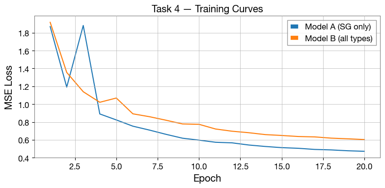
# --- Task 4: train Model A and Model B ---------------------------------------
print("Training Model A (sine-Gaussian only)...")
model_A = UNET2D(in_channels=2, out_channels=2, features=[32, 64, 128, 256]).to(DEVICE)
trl_A, vll_A = _train_stft(model_A, ld_A_tr, ld_A_vl)

print("\nTraining Model B (all 5 types)...")
model_B = UNET2D(in_channels=2, out_channels=2, features=[32, 64, 128, 256]).to(DEVICE)
trl_B, vll_B = _train_stft(model_B, ld_B_tr, ld_B_vl)

_plot_val_curves(
    {"Model A (SG only)": (trl_A, vll_A), "Model B (all types)": (trl_B, vll_B)},
    title="Task 4 — Training Curves",
)

Training Model A (sine-Gaussian only)...

Training on batch: 100%|██████████| 32/32 [00:10<00:00,  3.08it/s, loss=1.63]

Validation Loss: 1.869497
  ep  1/20  train=2.07405  val=1.86950

Training on batch: 100%|██████████| 32/32 [00:10<00:00,  3.12it/s, loss=1.14]

Validation Loss: 1.190895
  ep  2/20  train=1.39088  val=1.19090

Training on batch: 100%|██████████| 32/32 [00:10<00:00,  3.14it/s, loss=1.06]

Validation Loss: 1.882128
  ep  3/20  train=1.08695  val=1.88213

Training on batch: 100%|██████████| 32/32 [00:10<00:00,  3.14it/s, loss=0.928]

Validation Loss: 0.890039
  ep  4/20  train=0.93258  val=0.89004

Training on batch: 100%|██████████| 32/32 [00:10<00:00,  3.20it/s, loss=0.758]

Validation Loss: 0.822928
  ep  5/20  train=0.83083  val=0.82293

Training on batch: 100%|██████████| 32/32 [00:10<00:00,  3.15it/s, loss=0.767]

Validation Loss: 0.753019
  ep  6/20  train=0.76239  val=0.75302

Training on batch: 100%|██████████| 32/32 [00:10<00:00,  3.12it/s, loss=0.733]

Validation Loss: 0.709294
  ep  7/20  train=0.71413  val=0.70929

Training on batch: 100%|██████████| 32/32 [00:10<00:00,  3.14it/s, loss=0.56]

Validation Loss: 0.661775
  ep  8/20  train=0.66847  val=0.66177

Training on batch: 100%|██████████| 32/32 [00:10<00:00,  3.07it/s, loss=0.729]

Validation Loss: 0.618237
  ep  9/20  train=0.63769  val=0.61824

Training on batch: 100%|██████████| 32/32 [00:10<00:00,  3.06it/s, loss=0.661]

Validation Loss: 0.596375
  ep 10/20  train=0.60891  val=0.59638

Training on batch: 100%|██████████| 32/32 [00:10<00:00,  3.05it/s, loss=0.548]

Validation Loss: 0.572648
  ep 11/20  train=0.58531  val=0.57265

Training on batch: 100%|██████████| 32/32 [00:10<00:00,  2.93it/s, loss=0.718]

Validation Loss: 0.566103
  ep 12/20  train=0.56936  val=0.56610

Training on batch: 100%|██████████| 32/32 [00:11<00:00,  2.80it/s, loss=0.576]

Validation Loss: 0.541997
  ep 13/20  train=0.55485  val=0.54200

Training on batch: 100%|██████████| 32/32 [00:11<00:00,  2.67it/s, loss=0.582]

Validation Loss: 0.525553
  ep 14/20  train=0.53864  val=0.52555

Training on batch: 100%|██████████| 32/32 [00:12<00:00,  2.49it/s, loss=0.531]

Validation Loss: 0.512312
  ep 15/20  train=0.52329  val=0.51231

Training on batch: 100%|██████████| 32/32 [00:13<00:00,  2.44it/s, loss=0.554]

Validation Loss: 0.505129
  ep 16/20  train=0.51192  val=0.50513

Training on batch: 100%|██████████| 32/32 [00:13<00:00,  2.40it/s, loss=0.463]

Validation Loss: 0.492219
  ep 17/20  train=0.50049  val=0.49222

Training on batch: 100%|██████████| 32/32 [00:13<00:00,  2.35it/s, loss=0.397]

Validation Loss: 0.486816
  ep 18/20  train=0.48993  val=0.48682

Training on batch: 100%|██████████| 32/32 [00:13<00:00,  2.29it/s, loss=0.528]

Validation Loss: 0.477304
  ep 19/20  train=0.48497  val=0.47730

Training on batch: 100%|██████████| 32/32 [00:13<00:00,  2.33it/s, loss=0.45]

Validation Loss: 0.471514
  ep 20/20  train=0.47695  val=0.47151

Training Model B (all 5 types)...

Training on batch: 100%|██████████| 32/32 [00:13<00:00,  2.29it/s, loss=1.73]

Validation Loss: 1.917284
  ep  1/20  train=2.11746  val=1.91728

Training on batch: 100%|██████████| 32/32 [00:13<00:00,  2.45it/s, loss=1.33]

Validation Loss: 1.355619
  ep  2/20  train=1.52965  val=1.35562

Training on batch: 100%|██████████| 32/32 [00:12<00:00,  2.47it/s, loss=1.06]

Validation Loss: 1.139033
  ep  3/20  train=1.23486  val=1.13903

Training on batch: 100%|██████████| 32/32 [00:13<00:00,  2.43it/s, loss=0.993]

Validation Loss: 1.020941
  ep  4/20  train=1.06781  val=1.02094

Training on batch: 100%|██████████| 32/32 [00:13<00:00,  2.43it/s, loss=1.21]

Validation Loss: 1.068545
  ep  5/20  train=0.98438  val=1.06855

Training on batch: 100%|██████████| 32/32 [00:12<00:00,  2.47it/s, loss=1.01]

Validation Loss: 0.891574
  ep  6/20  train=0.92101  val=0.89157

Training on batch: 100%|██████████| 32/32 [00:12<00:00,  2.48it/s, loss=0.797]

Validation Loss: 0.859295
  ep  7/20  train=0.86210  val=0.85929

Training on batch: 100%|██████████| 32/32 [00:12<00:00,  2.50it/s, loss=0.694]

Validation Loss: 0.819899
  ep  8/20  train=0.81786  val=0.81990

Training on batch: 100%|██████████| 32/32 [00:12<00:00,  2.47it/s, loss=0.811]

Validation Loss: 0.778027
  ep  9/20  train=0.78551  val=0.77803

Training on batch: 100%|██████████| 32/32 [00:12<00:00,  2.49it/s, loss=0.858]

Validation Loss: 0.773908
  ep 10/20  train=0.75547  val=0.77391

Training on batch: 100%|██████████| 32/32 [00:13<00:00,  2.42it/s, loss=0.638]

Validation Loss: 0.721378
  ep 11/20  train=0.73188  val=0.72138

Training on batch: 100%|██████████| 32/32 [00:13<00:00,  2.40it/s, loss=0.652]

Validation Loss: 0.696435
  ep 12/20  train=0.70620  val=0.69644

Training on batch: 100%|██████████| 32/32 [00:13<00:00,  2.42it/s, loss=0.735]

Validation Loss: 0.679901
  ep 13/20  train=0.68718  val=0.67990

Training on batch: 100%|██████████| 32/32 [00:13<00:00,  2.37it/s, loss=0.801]

Validation Loss: 0.658621
  ep 14/20  train=0.67194  val=0.65862

Training on batch: 100%|██████████| 32/32 [00:13<00:00,  2.44it/s, loss=0.622]

Validation Loss: 0.648763
  ep 15/20  train=0.65335  val=0.64876

Training on batch: 100%|██████████| 32/32 [00:13<00:00,  2.38it/s, loss=0.666]

Validation Loss: 0.637170
  ep 16/20  train=0.64257  val=0.63717

Training on batch: 100%|██████████| 32/32 [00:13<00:00,  2.32it/s, loss=0.558]

Validation Loss: 0.632703
  ep 17/20  train=0.62989  val=0.63270

Training on batch: 100%|██████████| 32/32 [00:13<00:00,  2.32it/s, loss=0.547]

Validation Loss: 0.618770
  ep 18/20  train=0.61973  val=0.61877

Training on batch: 100%|██████████| 32/32 [00:13<00:00,  2.40it/s, loss=0.607]

Validation Loss: 0.611349
  ep 19/20  train=0.61335  val=0.61135

Training on batch: 100%|██████████| 32/32 [00:13<00:00,  2.35it/s, loss=0.59]

Validation Loss: 0.602976
  ep 20/20  train=0.60485  val=0.60298

../_images/notebooks_training_tutorial_colab_34_81.png

[31]:

# --- Task 4: in-sample test (sine-Gaussians) ---------------------------------
mm_A_sg = _mismatch_stft(model_A)
mm_B_sg = _mismatch_stft(model_B)
print(f"In-sample (sine-Gaussians):")
print(f"  Model A: {mm_A_sg*100:.2f} %   Model B: {mm_B_sg*100:.2f} %")

# --- Out-of-sample: ringdown glitches (no extra install needed) ---------------
_oos_noise = generate_gaussian_noise(mean, std_dev, 30, (LENGTH,), bilby_noise=False)
_T_OOS = T / 2
_oos_noisy_list, _oos_inj_list = [], []
for _n in _oos_noise:
    _, _rd = _gen_rd(duration=np.random.uniform(0.125, T))
    _rd = _rd - np.mean(_rd)
    _rd = whitened_snr_scaling(_rd, snr=np.random.uniform(30, 100))
    _L  = len(_rd)
    _i0 = int(_T_OOS * SAMPLE_RATE) - _L // 2
    if _i0 < 0 or _i0 + _L > LENGTH:
        continue
    _nn = _n.copy()
    _nn[_i0:_i0 + _L] += _rd
    _ij = np.zeros(LENGTH)
    _ij[_i0:_i0 + _L] = _rd
    _oos_noisy_list.append(_nn)
    _oos_inj_list.append(_ij)
_oos_n  = np.array(_oos_noisy_list)
_oos_ij = np.array(_oos_inj_list)

mm_A_rd = float(np.mean([
    1 - overlap(ij, reconstruct(n, model_A, scaler, DEVICE, N_FFT, HOP_LENGTH, WIN_LENGTH))
    for n, ij in zip(_oos_n, _oos_ij)
]))
mm_B_rd = float(np.mean([
    1 - overlap(ij, reconstruct(n, model_B, scaler, DEVICE, N_FFT, HOP_LENGTH, WIN_LENGTH))
    for n, ij in zip(_oos_n, _oos_ij)
]))
print(f"Out-of-sample (ringdowns):")
print(f"  Model A: {mm_A_rd*100:.2f} %   Model B: {mm_B_rd*100:.2f} %")

# --- Optional: gengli blip glitches ------------------------------------------
mm_A_bl = mm_B_bl = None
if GENGLI_AVAILABLE:
    import gengli as _gengli
    _ggen   = _gengli.glitch_generator("H1")
    _bl_noisy_list, _bl_inj_list = [], []
    for _n in _oos_noise[:20]:
        _blip = np.array(_ggen.get_glitch(1, srate=4096, snr=10, alpha=0.2, fhigh=1024)).squeeze()
        _blip = _blip - np.mean(_blip)
        _blip = whitened_snr_scaling(_blip, snr=30)
        _L    = min(len(_blip), LENGTH)
        _i0   = max(0, int(_T_OOS * SAMPLE_RATE) - _L // 2)
        _i0   = min(_i0, LENGTH - _L)
        _nn   = _n.copy()
        _nn[_i0:_i0 + _L]  += _blip[:_L]
        _ij = np.zeros(LENGTH)
        _ij[_i0:_i0 + _L]   = _blip[:_L]
        _bl_noisy_list.append(_nn)
        _bl_inj_list.append(_ij)
    _bl_n  = np.array(_bl_noisy_list)
    _bl_ij = np.array(_bl_inj_list)
    mm_A_bl = float(np.mean([
        1 - overlap(ij, reconstruct(n, model_A, scaler, DEVICE, N_FFT, HOP_LENGTH, WIN_LENGTH))
        for n, ij in zip(_bl_n, _bl_ij)
    ]))
    mm_B_bl = float(np.mean([
        1 - overlap(ij, reconstruct(n, model_B, scaler, DEVICE, N_FFT, HOP_LENGTH, WIN_LENGTH))
        for n, ij in zip(_bl_n, _bl_ij)
    ]))
    print(f"Out-of-sample (gengli blips, raw samples treated as training-rate data):")
    print(f"  Model A: {mm_A_bl*100:.2f} %   Model B: {mm_B_bl*100:.2f} %")
else:
    print("(gengli not installed — blip test skipped)")

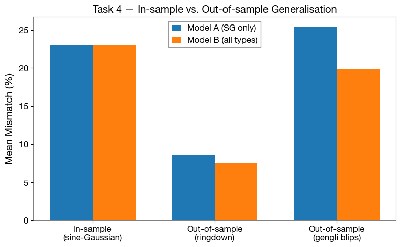
In-sample (sine-Gaussians):
  Model A: 23.05 %   Model B: 23.06 %
Generating pycbc noise...
Out-of-sample (ringdowns):
  Model A: 8.60 %   Model B: 7.56 %

/opt/homebrew/Caskroom/miniforge/base/envs/deepextractor/lib/python3.12/site-packages/gengli/glitch_generator.py:90: FutureWarning: You are using `torch.load` with `weights_only=False` (the current default value), which uses the default pickle module implicitly. It is possible to construct malicious pickle data which will execute arbitrary code during unpickling (See https://github.com/pytorch/pytorch/blob/main/SECURITY.md#untrusted-models for more details). In a future release, the default value for `weights_only` will be flipped to `True`. This limits the functions that could be executed during unpickling. Arbitrary objects will no longer be allowed to be loaded via this mode unless they are explicitly allowlisted by the user via `torch.serialization.add_safe_globals`. We recommend you start setting `weights_only=True` for any use case where you don't have full control of the loaded file. Please open an issue on GitHub for any issues related to this experimental feature.
  dict_weights = torch.load(weight_file, map_location = self.device)

Out-of-sample (gengli blips, raw samples treated as training-rate data):
  Model A: 25.43 %   Model B: 19.87 %

[32]:

# Task 4 summary: grouped bar chart
_cats = ["In-sample\n(sine-Gaussian)", "Out-of-sample\n(ringdown)"]
_mA   = [mm_A_sg * 100, mm_A_rd * 100]
_mB   = [mm_B_sg * 100, mm_B_rd * 100]

if mm_A_bl is not None:
    _cats.append("Out-of-sample\n(gengli blips)")
    _mA.append(mm_A_bl * 100)
    _mB.append(mm_B_bl * 100)

x   = np.arange(len(_cats))
w   = 0.35
fig, ax = plt.subplots(figsize=(8, 5))
ax.bar(x - w / 2, _mA, w, label="Model A (SG only)", color="C0")
ax.bar(x + w / 2, _mB, w, label="Model B (all types)", color="C1")
ax.set_xticks(x)
ax.set_xticklabels(_cats)
ax.set_ylabel("Mean Mismatch (%)")
ax.set_title("Task 4 — In-sample vs. Out-of-sample Generalisation")
ax.legend()
ax.grid(axis="y")
plt.tight_layout()
plt.show()

../_images/notebooks_training_tutorial_colab_36_0.png

[ ]:

[41]:

# --- Gengli blip: single reconstruction example (both models + ground truth) --
if GENGLI_AVAILABLE and len(_bl_n) > 0:
    _ex_noisy = _bl_n[0]
    _ex_inj   = _bl_ij[0]
    t_axis    = np.arange(LENGTH) * DT

    _r_A    = reconstruct(_ex_noisy, model_A, scaler, DEVICE, N_FFT, HOP_LENGTH, WIN_LENGTH)
    _r_B    = reconstruct(_ex_noisy, model_B, scaler, DEVICE, N_FFT, HOP_LENGTH, WIN_LENGTH)
    mm_ex_A = 1.0 - overlap(_ex_inj, _r_A)
    mm_ex_B = 1.0 - overlap(_ex_inj, _r_B)

    fig, ax = plt.subplots(figsize=(12, 4))
    ax.plot(t_axis, _ex_noisy, color="gray",  lw=0.8, alpha=0.4, label="Noisy input")
    ax.plot(t_axis, _r_A,     color="C0",    lw=1.5,
            label=f"Model A (SG only)   $\\mathcal{{M}}={mm_ex_A*100:.1f}\\%$")
    ax.plot(t_axis, _r_B,     color="C1",    lw=1.5,
            label=f"Model B (all types) $\\mathcal{{M}}={mm_ex_B*100:.1f}\\%$")
    ax.plot(t_axis, _ex_inj,  color="black", lw=1.5, ls="--", alpha=0.8,
            label="Injected (ground truth)")
    ax.set_title(
        f"Gengli blip reconstruction  —  "
        f"Model A $\\mathcal{{M}}={mm_ex_A*100:.1f}\\%$   "
        f"Model B $\\mathcal{{M}}={mm_ex_B*100:.1f}\\%$"
    )
    ax.set_xlabel("Time (s)")
    ax.set_ylabel("Amplitude")
    ax.legend(loc="lower right")
    ax.set_xlim(T_PHYSICAL / 2 - 2000, T_PHYSICAL / 2 + 2000)
    ax.grid(True)
    plt.tight_layout()
    plt.show()
else:
    print("gengli not available or no blip examples generated — skipping plot.")

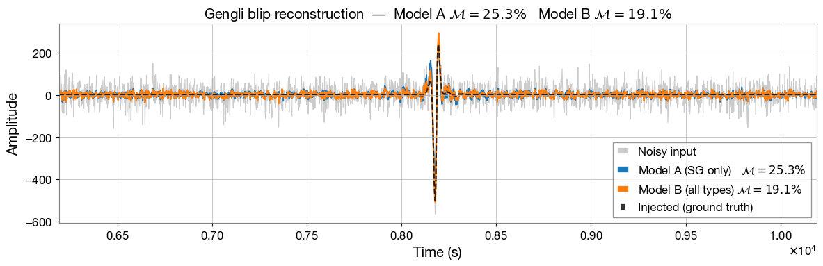
../_images/notebooks_training_tutorial_colab_38_0.png

[ ]: