DeepExtractor — Training Tutorial

This notebook trains a fresh DeepExtractor (U-Net 2D) model from scratch on a small synthetic (numpy) noise dataset, plots the training and validation losses, and then tests the trained model on held-out sine-Gaussian injections.

What synthetic noise means here: the background noise is white Gaussian noise scaled to match the variance of a whitened PyCBC noise realization (half the sampling rate). Use --bilby-noise / bilby_noise=True in order to train or use models corresponding to whitened detector noise aligning with theoretical O4 noise curves. In this case, the noise has zero mean and unit variance.

Pipeline overview:

1. Generate synthetic time-domain data (noisy glitch + background pairs)

2. Convert to STFT spectrograms (magnitude + phase)

3. Train the U-Net on spectrogram pairs

4. Plot losses

5. Test on sine-Gaussian injections

import os
import numpy as np
import torch
import torch.nn as nn
import torch.optim as optim
import matplotlib.pyplot as plt
from sklearn.preprocessing import StandardScaler
from torch.optim.lr_scheduler import ReduceLROnPlateau

import warnings
warnings.filterwarnings("ignore", "Wswiglal-redir-stdio")

from deepextractor.models.architectures import UNET2D
from deepextractor.generation.generate_timeseries import (
    generate_gaussian_noise, generate_synthetic_data, LENGTH, SAMPLE_RATE, T
)
from deepextractor.generation.glitch_functions import generate_sine_gaussian
from deepextractor.utils.signal import whitened_snr_scaling
from deepextractor.training.train_fn import train_fn
from deepextractor.utils.io import check_accuracy

Configuration

# Device — uses MPS on Apple Silicon, CUDA on Linux/Windows GPU, otherwise CPU
if torch.cuda.is_available():
    DEVICE = "cuda"
elif torch.backends.mps.is_available():
    DEVICE = "mps"
else:
    DEVICE = "cpu"
print(f"Using device: {DEVICE}")

# Dataset size — keep small for a quick demo; increase for real training
N_TRAIN = 1000
N_VAL   = 200

# Training
BATCH_SIZE              = 32
EPOCHS                  = 50    # maximum epochs; early stopping may stop sooner however, this specific architecture will likely converge at a much higher epoch
LR                      = 1e-4
LR_PATIENCE             = 4     # epochs without improvement before LR is reduced
LR_FACTOR               = 0.1   # factor to reduce LR by
EARLY_STOPPING_PATIENCE = 9     # epochs without improvement before training stops

# STFT parameters
# Original DeepExtractor (arXiv:2501.18423): N_FFT=512, WIN_LENGTH=64, HOP_LENGTH=32
# → produces (257, 257) spectrograms, richer time-frequency representation
#   but significantly slower to train.
# Tutorial default: smaller spectrograms for faster training, but still gives decent performance (please see 129x129 model in the paper).
N_FFT      = 256
WIN_LENGTH = N_FFT // 2
HOP_LENGTH = WIN_LENGTH // 2

Using device: mps

Step 1 — Generate synthetic time-domain data

Each training sample is a pair:

• Input glitch: background noise with 1–30 synthetic signal injections (chirps, sine-Gaussians, etc.)

• Target background: the same noise without any injections

The model learns to map glitchy strain → clean background.

mean, std_dev = 0, np.sqrt(SAMPLE_RATE / 2)  # PyCBC convention: variance = SAMPLE_RATE / 2

print("Generating training noise...")
train_noise = generate_gaussian_noise(mean, std_dev, N_TRAIN, (LENGTH,), bilby_noise=False)
print("Generating validation noise...")
val_noise   = generate_gaussian_noise(mean, std_dev, N_VAL,   (LENGTH,), bilby_noise=False)

print("Generating training pairs...")
glitch_train, bg_train = generate_synthetic_data(train_noise, bilby_noise=False, phase="train")
print("Generating validation pairs...")
glitch_val,   bg_val   = generate_synthetic_data(val_noise,   bilby_noise=False, phase="val")

print(f"\nTrain: {glitch_train.shape}  |  Val: {glitch_val.shape}")

Step 2 — Scale and convert to spectrograms

scaler = StandardScaler()
glitch_train_scaled = scaler.fit_transform(glitch_train.reshape(-1, 1)).reshape(glitch_train.shape)
bg_train_scaled     = scaler.transform(bg_train.reshape(-1, 1)).reshape(bg_train.shape)
glitch_val_scaled   = scaler.transform(glitch_val.reshape(-1, 1)).reshape(glitch_val.shape)
bg_val_scaled       = scaler.transform(bg_val.reshape(-1, 1)).reshape(bg_val.shape)

# Uncomment to save the scaler for use outside this notebook
# import pickle, os
# os.makedirs('/tmp/de_training_tutorial', exist_ok=True)
# with open('/tmp/de_training_tutorial/scaler.pkl', 'wb') as f:
#     pickle.dump(scaler, f)

# Convert to STFT spectrograms (in-memory)
window = torch.hann_window(WIN_LENGTH)

def to_mag_phase(arrays):
    """Convert a numpy array (N, time) to a (N, 2, F, T) mag/phase tensor."""
    t = torch.tensor(arrays, dtype=torch.float32)
    stft = torch.stft(t, n_fft=N_FFT, hop_length=HOP_LENGTH, win_length=WIN_LENGTH,
                      window=window, return_complex=True)
    mag   = torch.abs(stft)
    phase = torch.angle(stft)
    return torch.stack([mag, phase], dim=1)  # (N, 2, F, T)

glitch_train_spec = to_mag_phase(glitch_train_scaled)
bg_train_spec     = to_mag_phase(bg_train_scaled)
glitch_val_spec   = to_mag_phase(glitch_val_scaled)
bg_val_spec       = to_mag_phase(bg_val_scaled)

print(f"Spectrogram shape: {glitch_train_spec.shape}  — (N, 2, freq_bins, time_bins)")

# Uncomment to save spectrograms to disk (useful for large datasets or re-use)
# os.makedirs('/tmp/de_training_tutorial/spectrogram_domain', exist_ok=True)
# for name, arr in [
#     ('glitch_train_scaled_mag_phase',     glitch_train_spec.numpy()),
#     ('background_train_scaled_mag_phase', bg_train_spec.numpy()),
#     ('glitch_val_scaled_mag_phase',       glitch_val_spec.numpy()),
#     ('background_val_scaled_mag_phase',   bg_val_spec.numpy()),
# ]:
#     np.save(f'/tmp/de_training_tutorial/spectrogram_domain/{name}', arr)

Spectrogram shape: torch.Size([999, 2, 129, 129])  — (N, 2, freq_bins, time_bins)

Step 3 — Build model and data loaders

from torch.utils.data import TensorDataset, DataLoader

# Model architecture
# Original DeepExtractor (arXiv:2501.18423): features=[64, 128, 256, 512] — ~31M parameters.
# Use those to train a model equivalent to the published DeepExtractor.
# Tutorial default: one fewer layer and half the filters for faster training.
model = UNET2D(in_channels=2, out_channels=2, features=[32, 64, 128, 256]).to(DEVICE)
print(f"Model parameters: {sum(p.numel() for p in model.parameters()):,}")

train_ds = TensorDataset(glitch_train_spec, bg_train_spec)
val_ds   = TensorDataset(glitch_val_spec,   bg_val_spec)

train_loader = DataLoader(train_ds, batch_size=BATCH_SIZE, shuffle=True)
val_loader   = DataLoader(val_ds,   batch_size=BATCH_SIZE, shuffle=False)

print(f"Train batches: {len(train_loader)}  |  Val batches: {len(val_loader)}")
print(f"Spectrogram shape: {glitch_train_spec.shape}  — (N, 2, freq_bins, time_bins)")

Model parameters: 7,762,786
Train batches: 32  |  Val batches: 7
Spectrogram shape: torch.Size([999, 2, 129, 129])  — (N, 2, freq_bins, time_bins)

Step 4 — Train

We train the network for up to EPOCHS iterations. For this minimal tutorial configuration (1000 samples, reduced model), 50 epochs is sufficient to see the loss converge. To train a model to full convergence, set EPOCHS to a large number (e.g. 200) — the learning rate scheduler and early stopping will halt training automatically once the validation loss stops improving. For longer runs, we recommend using a CUDA GPU (e.g. Google Colab).

loss_fn   = nn.MSELoss()
optimizer = optim.Adam(model.parameters(), lr=LR)
scheduler = ReduceLROnPlateau(optimizer, mode="min", factor=LR_FACTOR, patience=LR_PATIENCE)
amp_scaler = torch.amp.GradScaler("cuda") if DEVICE == "cuda" else torch.amp.GradScaler("cpu")

train_losses, val_losses = [], []
best_val_loss           = float("inf")
early_stopping_counter  = 0

for epoch in range(EPOCHS):
    train_loss, _, _ = train_fn(
        train_loader, model, "DeepExtractor_257", optimizer, loss_fn, amp_scaler, DEVICE
    )
    val_loss, _, _ = check_accuracy(val_loader, model, "DeepExtractor_257", device=DEVICE)

    train_losses.append(train_loss)
    val_losses.append(val_loss)
    scheduler.step(val_loss)

    current_lr = optimizer.param_groups[0]['lr']
    print(f"Epoch {epoch+1:>3}/{EPOCHS}  train={train_loss:.5f}  val={val_loss:.5f}  lr={current_lr:.1e}")

    if val_loss < best_val_loss:
        best_val_loss          = val_loss
        early_stopping_counter = 0
    else:
        early_stopping_counter += 1
        if early_stopping_counter >= EARLY_STOPPING_PATIENCE:
            print(f"\nEarly stopping at epoch {epoch+1} (no improvement for {EARLY_STOPPING_PATIENCE} epochs).")
            break

print("\nTraining complete.")

Training on batch: 100%|██████████| 32/32 [00:21<00:00,  1.46it/s, loss=2.44]

Validation Loss: 2.545411
Epoch   1/50  train=2.80453  val=2.54541  lr=1.0e-04

Training on batch: 100%|██████████| 32/32 [00:14<00:00,  2.13it/s, loss=1.95]

Validation Loss: 1.898977
Epoch   2/50  train=2.11057  val=1.89898  lr=1.0e-04

Training on batch: 100%|██████████| 32/32 [00:15<00:00,  2.06it/s, loss=1.87]

Validation Loss: 1.739838
Epoch   3/50  train=1.76422  val=1.73984  lr=1.0e-04

Training on batch: 100%|██████████| 32/32 [00:15<00:00,  2.08it/s, loss=1.59]

Validation Loss: 1.527682
Epoch   4/50  train=1.58719  val=1.52768  lr=1.0e-04

Training on batch: 100%|██████████| 32/32 [00:15<00:00,  2.08it/s, loss=1.37]

Validation Loss: 1.414211
Epoch   5/50  train=1.45410  val=1.41421  lr=1.0e-04

Training on batch: 100%|██████████| 32/32 [00:15<00:00,  2.10it/s, loss=1.31]

Validation Loss: 1.315434
Epoch   6/50  train=1.35142  val=1.31543  lr=1.0e-04

Training on batch: 100%|██████████| 32/32 [00:15<00:00,  2.12it/s, loss=1.3]

Validation Loss: 1.250888
Epoch   7/50  train=1.26978  val=1.25089  lr=1.0e-04

Training on batch: 100%|██████████| 32/32 [00:15<00:00,  2.09it/s, loss=1.25]

Validation Loss: 1.190232
Epoch   8/50  train=1.20637  val=1.19023  lr=1.0e-04

Training on batch: 100%|██████████| 32/32 [00:15<00:00,  2.10it/s, loss=1.14]

Validation Loss: 1.114848
Epoch   9/50  train=1.14198  val=1.11485  lr=1.0e-04

Training on batch: 100%|██████████| 32/32 [00:15<00:00,  2.12it/s, loss=1.01]

Validation Loss: 1.045667
Epoch  10/50  train=1.08104  val=1.04567  lr=1.0e-04

Training on batch: 100%|██████████| 32/32 [00:15<00:00,  2.11it/s, loss=1.22]

Validation Loss: 1.002437
Epoch  11/50  train=1.03745  val=1.00244  lr=1.0e-04

Training on batch: 100%|██████████| 32/32 [00:15<00:00,  2.11it/s, loss=0.947]

Validation Loss: 0.969374
Epoch  12/50  train=0.98899  val=0.96937  lr=1.0e-04

Training on batch: 100%|██████████| 32/32 [00:15<00:00,  2.08it/s, loss=0.862]

Validation Loss: 0.923322
Epoch  13/50  train=0.95065  val=0.92332  lr=1.0e-04

Training on batch: 100%|██████████| 32/32 [00:15<00:00,  2.09it/s, loss=0.831]

Validation Loss: 0.903853
Epoch  14/50  train=0.91370  val=0.90385  lr=1.0e-04

Training on batch: 100%|██████████| 32/32 [00:15<00:00,  2.05it/s, loss=0.806]

Validation Loss: 0.870272
Epoch  15/50  train=0.88250  val=0.87027  lr=1.0e-04

Training on batch: 100%|██████████| 32/32 [00:15<00:00,  2.08it/s, loss=1]

Validation Loss: 0.840949
Epoch  16/50  train=0.86470  val=0.84095  lr=1.0e-04

Training on batch: 100%|██████████| 32/32 [00:15<00:00,  2.09it/s, loss=0.739]

Validation Loss: 0.810881
Epoch  17/50  train=0.82837  val=0.81088  lr=1.0e-04

Training on batch: 100%|██████████| 32/32 [00:15<00:00,  2.04it/s, loss=0.896]

Validation Loss: 0.790545
Epoch  18/50  train=0.80797  val=0.79054  lr=1.0e-04

Training on batch: 100%|██████████| 32/32 [00:15<00:00,  2.09it/s, loss=0.758]

Validation Loss: 0.770484
Epoch  19/50  train=0.78280  val=0.77048  lr=1.0e-04

Training on batch: 100%|██████████| 32/32 [00:15<00:00,  2.08it/s, loss=0.896]

Validation Loss: 0.750904
Epoch  20/50  train=0.76615  val=0.75090  lr=1.0e-04

Training on batch: 100%|██████████| 32/32 [00:15<00:00,  2.11it/s, loss=0.777]

Validation Loss: 0.730212
Epoch  21/50  train=0.74402  val=0.73021  lr=1.0e-04

Training on batch: 100%|██████████| 32/32 [00:15<00:00,  2.11it/s, loss=0.515]

Validation Loss: 0.718230
Epoch  22/50  train=0.72407  val=0.71823  lr=1.0e-04

Training on batch: 100%|██████████| 32/32 [00:15<00:00,  2.10it/s, loss=0.743]

Validation Loss: 0.699076
Epoch  23/50  train=0.71225  val=0.69908  lr=1.0e-04

Training on batch: 100%|██████████| 32/32 [00:15<00:00,  2.06it/s, loss=0.731]

Validation Loss: 0.679227
Epoch  24/50  train=0.69462  val=0.67923  lr=1.0e-04

Training on batch: 100%|██████████| 32/32 [00:15<00:00,  2.08it/s, loss=0.71]

Validation Loss: 0.666795
Epoch  25/50  train=0.67974  val=0.66680  lr=1.0e-04

Training on batch: 100%|██████████| 32/32 [00:15<00:00,  2.12it/s, loss=0.704]

Validation Loss: 0.652799
Epoch  26/50  train=0.66749  val=0.65280  lr=1.0e-04

Training on batch: 100%|██████████| 32/32 [00:15<00:00,  2.12it/s, loss=0.752]

Validation Loss: 0.652299
Epoch  27/50  train=0.66088  val=0.65230  lr=1.0e-04

Training on batch: 100%|██████████| 32/32 [00:15<00:00,  2.13it/s, loss=0.781]

Validation Loss: 0.635428
Epoch  28/50  train=0.64983  val=0.63543  lr=1.0e-04

Training on batch: 100%|██████████| 32/32 [00:15<00:00,  2.13it/s, loss=0.727]

Validation Loss: 0.627622
Epoch  29/50  train=0.63804  val=0.62762  lr=1.0e-04

Training on batch: 100%|██████████| 32/32 [00:15<00:00,  2.12it/s, loss=0.954]

Validation Loss: 0.618593
Epoch  30/50  train=0.63539  val=0.61859  lr=1.0e-04

Training on batch: 100%|██████████| 32/32 [00:15<00:00,  2.13it/s, loss=0.668]

Validation Loss: 0.611341
Epoch  31/50  train=0.62093  val=0.61134  lr=1.0e-04

Training on batch: 100%|██████████| 32/32 [00:15<00:00,  2.13it/s, loss=0.553]

Validation Loss: 0.602130
Epoch  32/50  train=0.61050  val=0.60213  lr=1.0e-04

Training on batch: 100%|██████████| 32/32 [00:15<00:00,  2.08it/s, loss=0.641]

Validation Loss: 0.595242
Epoch  33/50  train=0.60573  val=0.59524  lr=1.0e-04

Training on batch: 100%|██████████| 32/32 [00:15<00:00,  2.06it/s, loss=0.722]

Validation Loss: 0.591198
Epoch  34/50  train=0.60226  val=0.59120  lr=1.0e-04

Training on batch: 100%|██████████| 32/32 [00:15<00:00,  2.01it/s, loss=0.483]

Validation Loss: 0.586757
Epoch  35/50  train=0.59358  val=0.58676  lr=1.0e-04

Training on batch: 100%|██████████| 32/32 [00:15<00:00,  2.10it/s, loss=0.562]

Validation Loss: 0.579123
Epoch  36/50  train=0.58803  val=0.57912  lr=1.0e-04

Training on batch: 100%|██████████| 32/32 [00:15<00:00,  2.11it/s, loss=0.686]

Validation Loss: 0.574063
Epoch  37/50  train=0.58425  val=0.57406  lr=1.0e-04

Training on batch: 100%|██████████| 32/32 [00:15<00:00,  2.09it/s, loss=0.484]

Validation Loss: 0.571091
Epoch  38/50  train=0.57496  val=0.57109  lr=1.0e-04

Training on batch: 100%|██████████| 32/32 [00:15<00:00,  2.11it/s, loss=0.487]

Validation Loss: 0.565416
Epoch  39/50  train=0.57061  val=0.56542  lr=1.0e-04

Training on batch: 100%|██████████| 32/32 [00:15<00:00,  2.12it/s, loss=0.567]

Validation Loss: 0.561408
Epoch  40/50  train=0.56795  val=0.56141  lr=1.0e-04

Training on batch: 100%|██████████| 32/32 [00:15<00:00,  2.11it/s, loss=0.662]

Validation Loss: 0.557326
Epoch  41/50  train=0.56774  val=0.55733  lr=1.0e-04

Training on batch: 100%|██████████| 32/32 [00:15<00:00,  2.12it/s, loss=0.492]

Validation Loss: 0.555361
Epoch  42/50  train=0.55907  val=0.55536  lr=1.0e-04

Training on batch: 100%|██████████| 32/32 [00:15<00:00,  2.12it/s, loss=0.43]

Validation Loss: 0.553943
Epoch  43/50  train=0.55506  val=0.55394  lr=1.0e-04

Training on batch: 100%|██████████| 32/32 [00:15<00:00,  2.10it/s, loss=0.373]

Validation Loss: 0.551764
Epoch  44/50  train=0.55177  val=0.55176  lr=1.0e-04

Training on batch: 100%|██████████| 32/32 [00:15<00:00,  2.11it/s, loss=0.597]

Validation Loss: 0.546904
Epoch  45/50  train=0.55447  val=0.54690  lr=1.0e-04

Training on batch: 100%|██████████| 32/32 [00:15<00:00,  2.10it/s, loss=0.397]

Validation Loss: 0.544676
Epoch  46/50  train=0.54620  val=0.54468  lr=1.0e-04

Training on batch: 100%|██████████| 32/32 [00:15<00:00,  2.10it/s, loss=0.658]

Validation Loss: 0.542234
Epoch  47/50  train=0.55152  val=0.54223  lr=1.0e-04

Training on batch: 100%|██████████| 32/32 [00:15<00:00,  2.11it/s, loss=0.455]

Validation Loss: 0.540582
Epoch  48/50  train=0.54364  val=0.54058  lr=1.0e-04

Training on batch: 100%|██████████| 32/32 [00:15<00:00,  2.11it/s, loss=0.538]

Validation Loss: 0.539683
Epoch  49/50  train=0.54304  val=0.53968  lr=1.0e-04

Training on batch: 100%|██████████| 32/32 [00:15<00:00,  2.10it/s, loss=0.697]

Validation Loss: 0.537573
Epoch  50/50  train=0.54464  val=0.53757  lr=1.0e-04

Training complete.

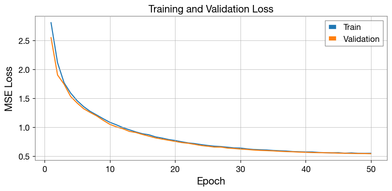
Step 5 — Plot losses

epochs_ran = range(1, len(train_losses) + 1)

fig, ax = plt.subplots(figsize=(8, 4))
ax.plot(epochs_ran, train_losses, label="Train",      color="C0")
ax.plot(epochs_ran, val_losses,   label="Validation", color="C1")
ax.set_xlabel("Epoch")
ax.set_ylabel("MSE Loss")
ax.set_title("Training and Validation Loss")
ax.legend()
ax.grid(True)
plt.tight_layout()
plt.show()

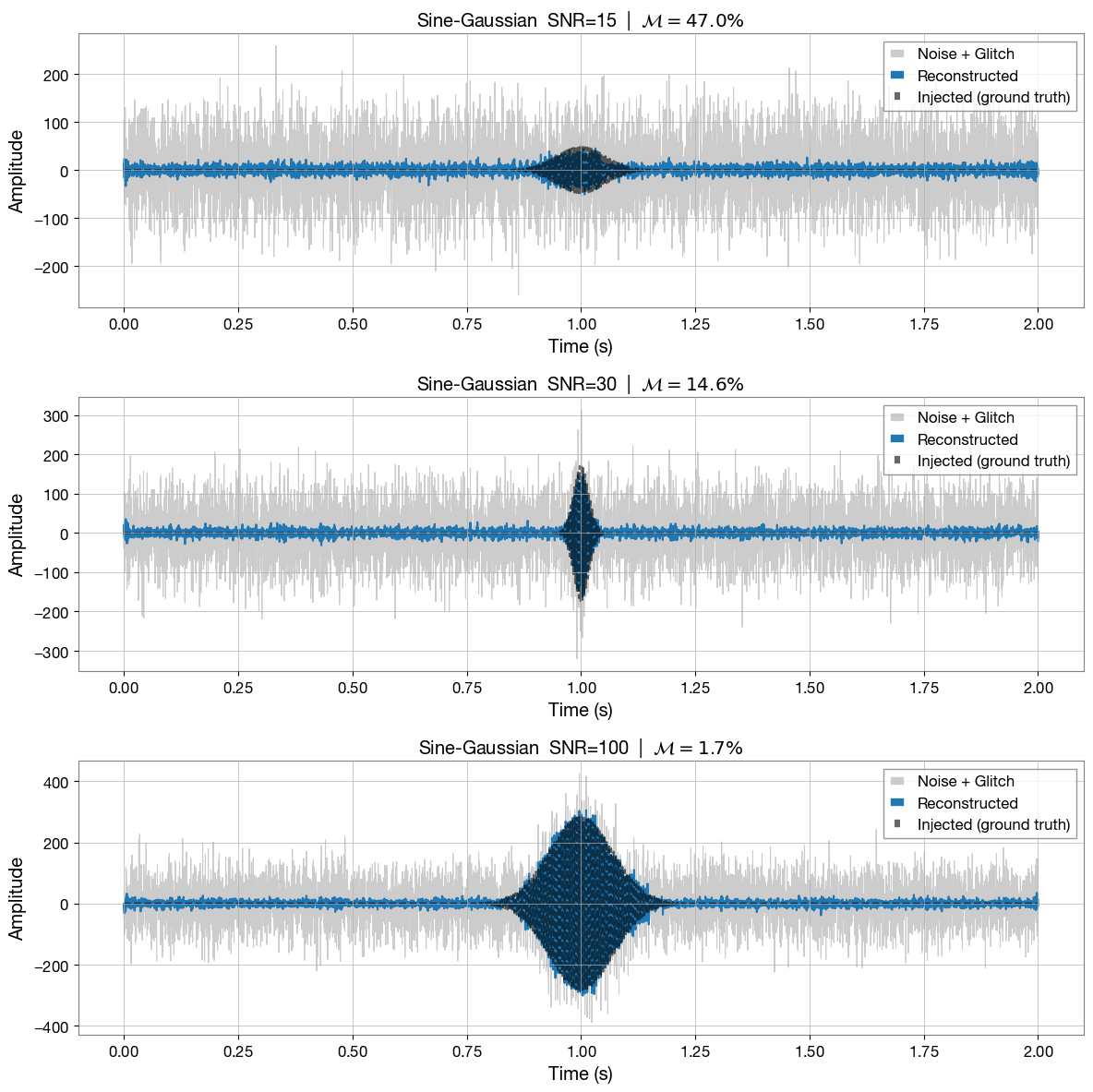
Step 6 — Test on sine-Gaussian injections

We generate fresh test examples — PyCBC (numpy) noise with a sine-Gaussian injected at a range of SNRs — and run them through the trained model. The model was never trained on these specific examples. We use three different test examples at three different SNRs, reporting the SNR and mismatch (\(\mathcal{M}\)) above each plot. Intuitively, the model better recovers louder glitches than quieter ones. The reconstructions below feature high-frequency artifacts as the model training did not fully converge, and it is a reduced architecture compared to the published version. Improved performance can be achieved by training this model until convergence or by modifying the layers of DeepExtractor’s U-Net to the published architecture, and increasing the resolution of the STFT spectrograms (please see above).

def reconstruct(noisy_signal, model, scaler, device, n_fft, hop_length, win_length):
    """Scale → STFT → U-Net → iSTFT → unscale → subtract background."""
    # Scale
    scaled = scaler.transform(noisy_signal.reshape(-1, 1)).reshape(noisy_signal.shape)

    # STFT
    window = torch.hann_window(win_length)
    t = torch.tensor(scaled, dtype=torch.float32).unsqueeze(0)  # (1, time)
    stft = torch.stft(t, n_fft=n_fft, hop_length=hop_length, win_length=win_length,
                      window=window, return_complex=True)
    mag   = torch.abs(stft)
    phase = torch.angle(stft)
    spec  = torch.stack([mag, phase], dim=1)  # (1, 2, F, T)

    # U-Net inference
    model.eval()
    with torch.no_grad():
        bg_spec = model(spec.to(device)).cpu()  # predicted background spectrogram

    # iSTFT
    bg_mag   = bg_spec[:, 0, :, :]
    bg_phase = bg_spec[:, 1, :, :]
    bg_complex = bg_mag * torch.exp(1j * bg_phase)
    bg_td = torch.istft(bg_complex, n_fft=n_fft, hop_length=hop_length,
                        win_length=win_length, window=window,
                        length=noisy_signal.shape[-1])

    # Unscale and subtract background to recover signal
    bg_unscaled = scaler.inverse_transform(bg_td.numpy().reshape(-1, 1)).reshape(-1)
    noisy_unscaled = noisy_signal.copy()
    reconstruction = noisy_unscaled - bg_unscaled
    return reconstruction

T_INJ = T / 2
SNR_VALUES = [15, 30, 100]

def overlap(a, b):
    """Normalised time-domain overlap (match) between two real signals.
    Equivalent to the PyCBC match on whitened data (flat PSD)."""
    return np.dot(a, b) / np.sqrt(np.dot(a, a) * np.dot(b, b))

fig, axes = plt.subplots(len(SNR_VALUES), 1, figsize=(12, 4 * len(SNR_VALUES)))
t_axis = np.linspace(0, T, LENGTH)

for ax, snr in zip(axes, SNR_VALUES):
    noise = generate_gaussian_noise(mean, std_dev, 1, (LENGTH,), bilby_noise=False)[0]

    # We set freq_max=256 when generating the sine-Gaussians for visualization purposes. This can be increased to the Nyquist frequency (i.e. freq_max=2048).
    _, wavelet = generate_sine_gaussian(duration=0.5, freq_max=256)
    wavelet = wavelet - np.mean(wavelet)
    wavelet = whitened_snr_scaling(wavelet, snr=snr)

    len_glitch = len(wavelet)
    id_start   = int(T_INJ * SAMPLE_RATE) - len_glitch // 2
    noisy      = noise.copy()
    noisy[id_start : id_start + len_glitch] += wavelet

    injected = np.zeros(LENGTH)
    injected[id_start : id_start + len_glitch] = wavelet

    reconstructed = reconstruct(noisy, model, scaler, DEVICE, N_FFT, HOP_LENGTH, WIN_LENGTH)

    match    = overlap(injected, reconstructed)
    mismatch = 1.0 - match

    ax.plot(t_axis, noisy,         color="gray",  lw=0.8, alpha=0.4, label="Noise + Glitch")
    ax.plot(t_axis, reconstructed, color="C0",    lw=1.5, label="Reconstructed")
    ax.plot(t_axis, injected,      color="black", lw=1.5, alpha=0.6, linestyle="--", label="Injected (ground truth)")
    ax.set_title(
        f"Sine-Gaussian  SNR={snr}  |  "
        f"$\\mathcal{{M}} = {mismatch*100:.1f} \% $"
    )
    ax.set_xlabel("Time (s)")
    ax.set_ylabel("Amplitude")
    ax.legend(loc="upper right")
    ax.grid(True)

plt.tight_layout()
plt.show()

<>:38: SyntaxWarning: invalid escape sequence '\%'
<>:38: SyntaxWarning: invalid escape sequence '\%'
/var/folders/xj/6sk96vdn15385fpjn9nd1rcw0000gp/T/ipykernel_22077/3874219395.py:38: SyntaxWarning: invalid escape sequence '\%'
  f"$\\mathcal{{M}} = {mismatch*100:.1f} \% $"

Generating pycbc noise...
Generating pycbc noise...
Generating pycbc noise...