DeepExtractor — Training Tutorial
This notebook trains a fresh DeepExtractor_257 (U-Net 2D) model from scratch on a small synthetic PyCBC noise dataset, plots the training and validation losses, and then tests the trained model on held-out sine-Gaussian injections.
What PyCBC noise means here: the background noise is white Gaussian noise scaled to match the variance of a whitened PyCBC noise realization. It is not coloured detector noise — use --bilby-noise / bilby_noise=True for that.
Pipeline overview:
Generate synthetic time-domain data (noisy glitch + background pairs)
Convert to STFT spectrograms (magnitude + phase)
Train the U-Net on spectrogram pairs
Plot losses
Test on sine-Gaussian injections
[1]:
import os
import numpy as np
import torch
import torch.nn as nn
import torch.optim as optim
import matplotlib.pyplot as plt
from sklearn.preprocessing import StandardScaler
from torch.optim.lr_scheduler import ReduceLROnPlateau

import warnings
warnings.filterwarnings("ignore", "Wswiglal-redir-stdio")

from deepextractor.models.architectures import UNET2D
from deepextractor.generation.generate_timeseries import (
    generate_gaussian_noise, generate_synthetic_data, LENGTH, SAMPLE_RATE, T
)
from deepextractor.generation.glitch_functions import generate_sine_gaussian
from deepextractor.utils.signal import whitened_snr_scaling
from deepextractor.training.train_fn import train_fn
from deepextractor.utils.io import check_accuracy
Configuration
[2]:
# Device — uses MPS on Apple Silicon, CUDA on Linux/Windows GPU, otherwise CPU
if torch.cuda.is_available():
    DEVICE = "cuda"
elif torch.backends.mps.is_available():
    DEVICE = "mps"
else:
    DEVICE = "cpu"
print(f"Using device: {DEVICE}")

# Dataset size — keep small for a quick demo; increase for real training
N_TRAIN = 1000
N_VAL   = 200

# Training
BATCH_SIZE              = 32
EPOCHS                  = 50    # maximum epochs; early stopping may stop sooner
LR                      = 1e-4
LR_PATIENCE             = 4     # epochs without improvement before LR is reduced
LR_FACTOR               = 0.1   # factor to reduce LR by
EARLY_STOPPING_PATIENCE = 9     # epochs without improvement before training stops

# STFT parameters
# Original DeepExtractor (arXiv:2501.18423): N_FFT=512, WIN_LENGTH=64, HOP_LENGTH=32
# → produces (257, 257) spectrograms, richer time-frequency representation
#   but significantly slower to train.
# Tutorial default: smaller spectrograms for faster training, but still gives decent performance (please see 129x129 model in the paper).
N_FFT      = 256
WIN_LENGTH = N_FFT // 2
HOP_LENGTH = WIN_LENGTH // 2
Using device: mps
Step 1 — Generate synthetic time-domain data
Each training sample is a pair:
Input
glitch: background noise with 1–30 synthetic signal injections (chirps, sine-Gaussians, etc.)Target
background: the same noise without any injections
The model learns to map glitchy strain → clean background.
[3]:
mean, std_dev = 0, np.sqrt(SAMPLE_RATE)

print("Generating training noise...")
train_noise = generate_gaussian_noise(mean, std_dev, N_TRAIN, (LENGTH,), bilby_noise=False)
print("Generating validation noise...")
val_noise   = generate_gaussian_noise(mean, std_dev, N_VAL,   (LENGTH,), bilby_noise=False)

print("Generating training pairs...")
glitch_train, bg_train = generate_synthetic_data(train_noise, bilby_noise=False, phase="train")
print("Generating validation pairs...")
glitch_val,   bg_val   = generate_synthetic_data(val_noise,   bilby_noise=False, phase="val")

print(f"\nTrain: {glitch_train.shape}  |  Val: {glitch_val.shape}")
Generating training noise...
Generating pycbc noise...
Generating validation noise...
Generating pycbc noise...
Generating training pairs...
Generating Synthetic Train Data: 100%|██████████| 1000/1000 [00:02<00:00, 453.94it/s]
Generating validation pairs...
Generating Synthetic Val Data: 100%|██████████| 200/200 [00:00<00:00, 374.51it/s]
Train: (1000, 8192) | Val: (200, 8192)
Step 2 — Scale and convert to spectrograms
[4]:
scaler = StandardScaler()
glitch_train_scaled = scaler.fit_transform(glitch_train.reshape(-1, 1)).reshape(glitch_train.shape)
bg_train_scaled     = scaler.transform(bg_train.reshape(-1, 1)).reshape(bg_train.shape)
glitch_val_scaled   = scaler.transform(glitch_val.reshape(-1, 1)).reshape(glitch_val.shape)
bg_val_scaled       = scaler.transform(bg_val.reshape(-1, 1)).reshape(bg_val.shape)

# Uncomment to save the scaler for use outside this notebook
# import pickle, os
# os.makedirs('/tmp/de_training_tutorial', exist_ok=True)
# with open('/tmp/de_training_tutorial/scaler.pkl', 'wb') as f:
#     pickle.dump(scaler, f)

# Convert to STFT spectrograms (in-memory)
window = torch.hann_window(WIN_LENGTH)

def to_mag_phase(arrays):
    """Convert a numpy array (N, time) to a (N, 2, F, T) mag/phase tensor."""
    t = torch.tensor(arrays, dtype=torch.float32)
    stft = torch.stft(t, n_fft=N_FFT, hop_length=HOP_LENGTH, win_length=WIN_LENGTH,
                      window=window, return_complex=True)
    mag   = torch.abs(stft)
    phase = torch.angle(stft)
    return torch.stack([mag, phase], dim=1)  # (N, 2, F, T)

glitch_train_spec = to_mag_phase(glitch_train_scaled)
bg_train_spec     = to_mag_phase(bg_train_scaled)
glitch_val_spec   = to_mag_phase(glitch_val_scaled)
bg_val_spec       = to_mag_phase(bg_val_scaled)

print(f"Spectrogram shape: {glitch_train_spec.shape}  — (N, 2, freq_bins, time_bins)")

# Uncomment to save spectrograms to disk (useful for large datasets or re-use)
# os.makedirs('/tmp/de_training_tutorial/spectrogram_domain', exist_ok=True)
# for name, arr in [
#     ('glitch_train_scaled_mag_phase',     glitch_train_spec.numpy()),
#     ('background_train_scaled_mag_phase', bg_train_spec.numpy()),
#     ('glitch_val_scaled_mag_phase',       glitch_val_spec.numpy()),
#     ('background_val_scaled_mag_phase',   bg_val_spec.numpy()),
# ]:
#     np.save(f'/tmp/de_training_tutorial/spectrogram_domain/{name}', arr)
Spectrogram shape: torch.Size([1000, 2, 129, 129]) — (N, 2, freq_bins, time_bins)
Step 3 — Build model and data loaders
[5]:
from torch.utils.data import TensorDataset, DataLoader

# Model architecture
# Original DeepExtractor (arXiv:2501.18423): features=[64, 128, 256, 512] — ~31M parameters.
# Use those to train a model equivalent to the published DeepExtractor.
# Tutorial default: one fewer layer and half the filters for faster training.
model = UNET2D(in_channels=2, out_channels=2, features=[32, 64, 128, 256]).to(DEVICE)
print(f"Model parameters: {sum(p.numel() for p in model.parameters()):,}")

train_ds = TensorDataset(glitch_train_spec, bg_train_spec)
val_ds   = TensorDataset(glitch_val_spec,   bg_val_spec)

train_loader = DataLoader(train_ds, batch_size=BATCH_SIZE, shuffle=True)
val_loader   = DataLoader(val_ds,   batch_size=BATCH_SIZE, shuffle=False)

print(f"Train batches: {len(train_loader)}  |  Val batches: {len(val_loader)}")
print(f"Spectrogram shape: {glitch_train_spec.shape}  — (N, 2, freq_bins, time_bins)")
Model parameters: 7,762,786
Train batches: 32  |  Val batches: 7
Spectrogram shape: torch.Size([1000, 2, 129, 129])  — (N, 2, freq_bins, time_bins)
Step 4 — Train
[6]:
loss_fn   = nn.MSELoss()
optimizer = optim.Adam(model.parameters(), lr=LR)
scheduler = ReduceLROnPlateau(optimizer, mode="min", factor=LR_FACTOR, patience=LR_PATIENCE)
amp_scaler = torch.amp.GradScaler("cuda") if DEVICE == "cuda" else torch.amp.GradScaler("cpu")

train_losses, val_losses = [], []
best_val_loss           = float("inf")
early_stopping_counter  = 0

for epoch in range(EPOCHS):
    train_loss, _, _ = train_fn(
        train_loader, model, "DeepExtractor_257", optimizer, loss_fn, amp_scaler, DEVICE
    )
    val_loss, _, _ = check_accuracy(val_loader, model, "DeepExtractor_257", device=DEVICE)

    train_losses.append(train_loss)
    val_losses.append(val_loss)
    scheduler.step(val_loss)

    current_lr = optimizer.param_groups[0]['lr']
    print(f"Epoch {epoch+1:>3}/{EPOCHS}  train={train_loss:.5f}  val={val_loss:.5f}  lr={current_lr:.1e}")

    if val_loss < best_val_loss:
        best_val_loss          = val_loss
        early_stopping_counter = 0
    else:
        early_stopping_counter += 1
        if early_stopping_counter >= EARLY_STOPPING_PATIENCE:
            print(f"\nEarly stopping at epoch {epoch+1} (no improvement for {EARLY_STOPPING_PATIENCE} epochs).")
            break

print("\nTraining complete.")
Training on batch: 100%|██████████| 32/32 [00:11<00:00, 2.83it/s, loss=1.95]
Validation Loss: 2.218210
Epoch   1/50  train=2.32153  val=2.21821  lr=1.0e-04
Training on batch: 100%|██████████| 32/32 [00:10<00:00, 3.05it/s, loss=1.54]
Validation Loss: 1.511046
Epoch   2/50  train=1.68615  val=1.51105  lr=1.0e-04
Training on batch: 100%|██████████| 32/32 [00:10<00:00, 3.02it/s, loss=1.22]
Validation Loss: 1.312862
Epoch   3/50  train=1.37830  val=1.31286  lr=1.0e-04
Training on batch: 100%|██████████| 32/32 [00:10<00:00, 3.04it/s, loss=1.27]
Validation Loss: 1.163939
Epoch   4/50  train=1.18296  val=1.16394  lr=1.0e-04
Training on batch: 100%|██████████| 32/32 [00:10<00:00, 3.10it/s, loss=0.918]
Validation Loss: 1.020379
Epoch   5/50  train=1.06407  val=1.02038  lr=1.0e-04
Training on batch: 100%|██████████| 32/32 [00:10<00:00, 3.10it/s, loss=0.928]
Validation Loss: 0.980715
Epoch   6/50  train=0.97128  val=0.98071  lr=1.0e-04
Training on batch: 100%|██████████| 32/32 [00:10<00:00, 3.06it/s, loss=0.951]
Validation Loss: 0.869840
Epoch   7/50  train=0.91569  val=0.86984  lr=1.0e-04
Training on batch: 100%|██████████| 32/32 [00:10<00:00, 3.04it/s, loss=0.877]
Validation Loss: 0.817595
Epoch   8/50  train=0.85876  val=0.81759  lr=1.0e-04
Training on batch: 100%|██████████| 32/32 [00:10<00:00, 3.01it/s, loss=0.706]
Validation Loss: 0.806517
Epoch   9/50  train=0.81324  val=0.80652  lr=1.0e-04
Training on batch: 100%|██████████| 32/32 [00:10<00:00, 2.93it/s, loss=0.732]
Validation Loss: 0.753120
Epoch  10/50  train=0.78160  val=0.75312  lr=1.0e-04
Training on batch: 100%|██████████| 32/32 [00:11<00:00, 2.89it/s, loss=0.743]
Validation Loss: 0.719149
Epoch  11/50  train=0.75014  val=0.71915  lr=1.0e-04
Training on batch: 100%|██████████| 32/32 [00:11<00:00, 2.80it/s, loss=0.76]
Validation Loss: 0.698354
Epoch  12/50  train=0.72427  val=0.69835  lr=1.0e-04
Training on batch: 100%|██████████| 32/32 [00:11<00:00, 2.69it/s, loss=0.601]
Validation Loss: 0.680848
Epoch  13/50  train=0.69808  val=0.68085  lr=1.0e-04
Training on batch: 100%|██████████| 32/32 [00:12<00:00, 2.59it/s, loss=0.682]
Validation Loss: 0.660272
Epoch  14/50  train=0.68013  val=0.66027  lr=1.0e-04
Training on batch: 100%|██████████| 32/32 [00:12<00:00, 2.50it/s, loss=0.595]
Validation Loss: 0.647760
Epoch  15/50  train=0.66030  val=0.64776  lr=1.0e-04
Training on batch: 100%|██████████| 32/32 [00:13<00:00, 2.43it/s, loss=0.686]
Validation Loss: 0.632859
Epoch  16/50  train=0.64636  val=0.63286  lr=1.0e-04
Training on batch: 100%|██████████| 32/32 [00:13<00:00, 2.40it/s, loss=0.585]
Validation Loss: 0.617714
Epoch  17/50  train=0.63055  val=0.61771  lr=1.0e-04
Training on batch: 100%|██████████| 32/32 [00:13<00:00, 2.44it/s, loss=0.729]
Validation Loss: 0.841430
Epoch  18/50  train=0.62186  val=0.84143  lr=1.0e-04
Training on batch: 100%|██████████| 32/32 [00:13<00:00, 2.46it/s, loss=0.575]
Validation Loss: 0.603988
Epoch  19/50  train=0.62017  val=0.60399  lr=1.0e-04
Training on batch: 100%|██████████| 32/32 [00:13<00:00, 2.45it/s, loss=0.646]
Validation Loss: 0.593803
Epoch  20/50  train=0.60578  val=0.59380  lr=1.0e-04
Training on batch: 100%|██████████| 32/32 [00:12<00:00, 2.48it/s, loss=0.629]
Validation Loss: 0.581474
Epoch  21/50  train=0.59351  val=0.58147  lr=1.0e-04
Training on batch: 100%|██████████| 32/32 [00:12<00:00, 2.50it/s, loss=0.575]
Validation Loss: 0.572586
Epoch  22/50  train=0.58487  val=0.57259  lr=1.0e-04
Training on batch: 100%|██████████| 32/32 [00:12<00:00, 2.52it/s, loss=0.645]
Validation Loss: 0.564201
Epoch  23/50  train=0.58049  val=0.56420  lr=1.0e-04
Training on batch: 100%|██████████| 32/32 [00:12<00:00, 2.51it/s, loss=0.73]
Validation Loss: 0.562453
Epoch  24/50  train=0.57640  val=0.56245  lr=1.0e-04
Training on batch: 100%|██████████| 32/32 [00:12<00:00, 2.52it/s, loss=0.725]
Validation Loss: 0.556875
Epoch  25/50  train=0.57033  val=0.55688  lr=1.0e-04
Training on batch: 100%|██████████| 32/32 [00:12<00:00, 2.51it/s, loss=0.604]
Validation Loss: 0.556285
Epoch  26/50  train=0.56327  val=0.55629  lr=1.0e-04
Training on batch: 100%|██████████| 32/32 [00:13<00:00, 2.36it/s, loss=0.475]
Validation Loss: 0.547908
Epoch  27/50  train=0.55664  val=0.54791  lr=1.0e-04
Training on batch: 100%|██████████| 32/32 [00:14<00:00, 2.19it/s, loss=0.487]
Validation Loss: 0.545304
Epoch  28/50  train=0.55267  val=0.54530  lr=1.0e-04
Training on batch: 100%|██████████| 32/32 [00:13<00:00, 2.44it/s, loss=0.504]
Validation Loss: 0.542404
Epoch  29/50  train=0.54966  val=0.54240  lr=1.0e-04
Training on batch: 100%|██████████| 32/32 [00:13<00:00, 2.44it/s, loss=0.455]
Validation Loss: 0.539977
Epoch  30/50  train=0.54552  val=0.53998  lr=1.0e-04
Training on batch: 100%|██████████| 32/32 [00:13<00:00, 2.32it/s, loss=0.641]
Validation Loss: 0.536445
Epoch  31/50  train=0.54668  val=0.53645  lr=1.0e-04
Training on batch: 100%|██████████| 32/32 [00:13<00:00, 2.40it/s, loss=0.534]
Validation Loss: 0.535496
Epoch  32/50  train=0.54160  val=0.53550  lr=1.0e-04
Training on batch: 100%|██████████| 32/32 [00:13<00:00, 2.42it/s, loss=0.608]
Validation Loss: 0.533340
Epoch  33/50  train=0.54091  val=0.53334  lr=1.0e-04
Training on batch: 100%|██████████| 32/32 [00:13<00:00, 2.43it/s, loss=0.613]
Validation Loss: 0.530971
Epoch  34/50  train=0.53817  val=0.53097  lr=1.0e-04
Training on batch: 100%|██████████| 32/32 [00:13<00:00, 2.31it/s, loss=0.42]
Validation Loss: 0.530778
Epoch  35/50  train=0.53090  val=0.53078  lr=1.0e-04
Training on batch: 100%|██████████| 32/32 [00:15<00:00, 2.06it/s, loss=0.641]
Validation Loss: 0.527804
Epoch  36/50  train=0.53390  val=0.52780  lr=1.0e-04
Training on batch: 100%|██████████| 32/32 [00:16<00:00, 1.95it/s, loss=0.527]
Validation Loss: 0.527331
Epoch  37/50  train=0.52809  val=0.52733  lr=1.0e-04
Training on batch: 100%|██████████| 32/32 [00:15<00:00, 2.13it/s, loss=0.664]
Validation Loss: 0.526076
Epoch  38/50  train=0.52855  val=0.52608  lr=1.0e-04
Training on batch: 100%|██████████| 32/32 [00:13<00:00, 2.31it/s, loss=0.641]
Validation Loss: 0.525271
Epoch  39/50  train=0.52609  val=0.52527  lr=1.0e-04
Training on batch: 100%|██████████| 32/32 [00:13<00:00, 2.34it/s, loss=0.409]
Validation Loss: 0.529516
Epoch  40/50  train=0.51858  val=0.52952  lr=1.0e-04
Training on batch: 100%|██████████| 32/32 [00:13<00:00, 2.34it/s, loss=0.44]
Validation Loss: 0.523367
Epoch  41/50  train=0.51629  val=0.52337  lr=1.0e-04
Training on batch: 100%|██████████| 32/32 [00:13<00:00, 2.35it/s, loss=0.568]
Validation Loss: 0.522603
Epoch  42/50  train=0.51454  val=0.52260  lr=1.0e-04
Training on batch: 100%|██████████| 32/32 [00:13<00:00, 2.36it/s, loss=0.557]
Validation Loss: 0.521652
Epoch  43/50  train=0.51073  val=0.52165  lr=1.0e-04
Training on batch: 100%|██████████| 32/32 [00:14<00:00, 2.27it/s, loss=0.514]
Validation Loss: 0.521917
Epoch  44/50  train=0.50676  val=0.52192  lr=1.0e-04
Training on batch: 100%|██████████| 32/32 [00:13<00:00, 2.37it/s, loss=0.467]
Validation Loss: 0.520662
Epoch  45/50  train=0.50248  val=0.52066  lr=1.0e-04
Training on batch: 100%|██████████| 32/32 [00:13<00:00, 2.29it/s, loss=0.586]
Validation Loss: 0.521084
Epoch  46/50  train=0.50213  val=0.52108  lr=1.0e-04
Training on batch: 100%|██████████| 32/32 [00:13<00:00, 2.29it/s, loss=0.424]
Validation Loss: 0.520615
Epoch  47/50  train=0.49446  val=0.52061  lr=1.0e-04
Training on batch: 100%|██████████| 32/32 [00:13<00:00, 2.37it/s, loss=0.399]
Validation Loss: 0.521620
Epoch  48/50  train=0.48950  val=0.52162  lr=1.0e-04
Training on batch: 100%|██████████| 32/32 [00:13<00:00, 2.32it/s, loss=0.521]
Validation Loss: 0.520201
Epoch  49/50  train=0.48736  val=0.52020  lr=1.0e-04
Training on batch: 100%|██████████| 32/32 [00:13<00:00, 2.33it/s, loss=0.614]
Validation Loss: 0.521240
Epoch  50/50  train=0.48693  val=0.52124  lr=1.0e-04

Training complete.
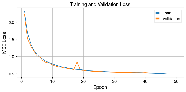
Step 5 — Plot losses
[7]:
epochs_ran = range(1, len(train_losses) + 1)

fig, ax = plt.subplots(figsize=(8, 4))
ax.plot(epochs_ran, train_losses, label="Train",      color="C0")
ax.plot(epochs_ran, val_losses,   label="Validation", color="C1")
ax.set_xlabel("Epoch")
ax.set_ylabel("MSE Loss")
ax.set_title("Training and Validation Loss")
ax.legend()
ax.grid(True)
plt.tight_layout()
plt.show()
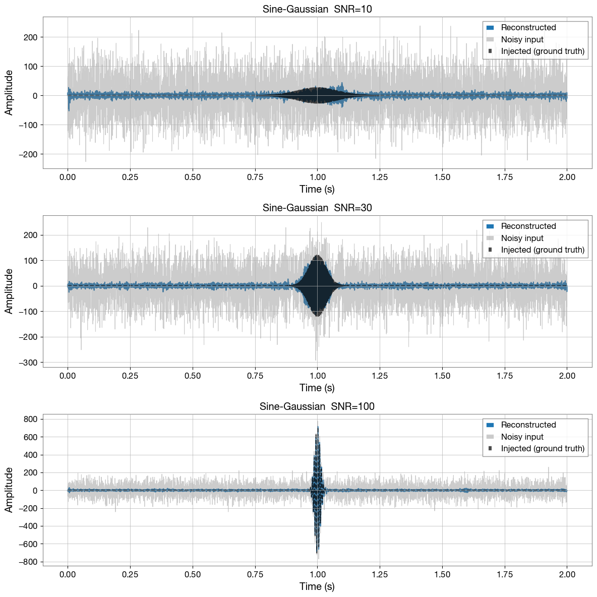
Step 6 — Test on sine-Gaussian injections
We generate fresh test examples — PyCBC (numpy) noise with a sine-Gaussian injected at a range of SNRs — and run them through the trained model. The model was never trained on these specific examples.
[8]:
def reconstruct(noisy_signal, model, scaler, device, n_fft, hop_length, win_length):
    """Scale → STFT → U-Net → iSTFT → unscale → subtract background."""
    # Scale
    scaled = scaler.transform(noisy_signal.reshape(-1, 1)).reshape(noisy_signal.shape)

    # STFT
    window = torch.hann_window(win_length)
    t = torch.tensor(scaled, dtype=torch.float32).unsqueeze(0)  # (1, time)
    stft = torch.stft(t, n_fft=n_fft, hop_length=hop_length, win_length=win_length,
                      window=window, return_complex=True)
    mag   = torch.abs(stft)
    phase = torch.angle(stft)
    spec  = torch.stack([mag, phase], dim=1)  # (1, 2, F, T)

    # U-Net inference
    model.eval()
    with torch.no_grad():
        bg_spec = model(spec.to(device)).cpu()  # predicted background spectrogram

    # iSTFT
    bg_mag   = bg_spec[:, 0, :, :]
    bg_phase = bg_spec[:, 1, :, :]
    bg_complex = bg_mag * torch.exp(1j * bg_phase)
    bg_td = torch.istft(bg_complex, n_fft=n_fft, hop_length=hop_length,
                        win_length=win_length, window=window,
                        length=noisy_signal.shape[-1])

    # Unscale and subtract background to recover signal
    bg_unscaled = scaler.inverse_transform(bg_td.numpy().reshape(-1, 1)).reshape(-1)
    noisy_unscaled = noisy_signal.copy()
    reconstruction = noisy_unscaled - bg_unscaled
    return reconstruction
[10]:
T_INJ = T / 2
SNR_VALUES = [10, 30, 100]

def overlap(a, b):
    """Normalised time-domain overlap (match) between two real signals.
    Equivalent to the PyCBC match on whitened data (flat PSD)."""
    return np.dot(a, b) / np.sqrt(np.dot(a, a) * np.dot(b, b))

fig, axes = plt.subplots(len(SNR_VALUES), 1, figsize=(12, 4 * len(SNR_VALUES)))
t_axis = np.linspace(0, T, LENGTH)

for ax, snr in zip(axes, SNR_VALUES):
    noise = generate_gaussian_noise(mean, std_dev, 1, (LENGTH,), bilby_noise=False)[0]

    _, wavelet = generate_sine_gaussian(duration=0.5, freq_max=1024)
    wavelet = wavelet - np.mean(wavelet)
    wavelet = whitened_snr_scaling(wavelet, snr=snr)

    len_glitch = len(wavelet)
    id_start   = int(T_INJ * SAMPLE_RATE) - len_glitch // 2
    noisy      = noise.copy()
    noisy[id_start : id_start + len_glitch] += wavelet

    injected = np.zeros(LENGTH)
    injected[id_start : id_start + len_glitch] = wavelet

    reconstructed = reconstruct(noisy, model, scaler, DEVICE, N_FFT, HOP_LENGTH, WIN_LENGTH)

    match    = overlap(injected, reconstructed)
    mismatch = 1.0 - match

    ax.plot(t_axis, injected,      color="black", lw=1.5, linestyle="--", label="Injected (ground truth)")
    ax.plot(t_axis, reconstructed, color="C0",    lw=1.5, label="Reconstructed")
    ax.plot(t_axis, noisy,         color="gray",  lw=0.8, alpha=0.4, label="Noisy input")
    ax.set_title(
        f"Sine-Gaussian  SNR={snr}  |  "
        f"Match $= {match:.3f}$,  $\\mathcal{{M}} = {mismatch:.3f}$"
    )
    ax.set_xlabel("Time (s)")
    ax.set_ylabel("Amplitude")
    ax.legend(loc="upper right")
    ax.grid(True)

plt.tight_layout()
plt.show()
Generating pycbc noise...
Generating pycbc noise...
Generating pycbc noise...
[ ]: